Research and analysis

Estimates of the impact of IPS over 12 months: Health-led Employment Trial Evaluation

Updated 8 April 2024

Applies to England, Scotland and Wales

DWP research report no.1034

A report of research carried out by the Institute for Employment Studies on behalf of the Department for Work and Pensions.

You may re-use this information (not including logos) free of charge in any format or medium, under the terms of the Open Government Licence.

To view this licence, visit the National Archives

Or write to:

Information Policy Team
The National Archives
Kew
London
TW9 4DU

Email: psi@nationalarchives.gov.uk

This document/publication is also available on our website at: Research at DWP

If you would like to know more about DWP research, email: socialresearch@dwp.gov.uk

First published July 2023.

ISBN 978-1-78659-546-1

Views expressed in this report are not necessarily those of the Department for Work and Pensions or any other government department.

Executive summary

This report provides detailed insights into the 12-month impacts for the health-led employment trials (HLTs). The analysis demonstrated:

• among those in WMCA, there was a positive impact on employment, significant at the 99% confidence level. The treatment group were 4 percentage points more likely to have been in work for 13 or more weeks in the year following randomisation than the control group. However, there were no significant impacts on earnings, or health and wellbeing outcomes.
• for the SCR out-of-work (OOW) group, being assigned to the treatment group had no statistically significant effect on either employment or earnings. Small positive impacts were seen for health and wellbeing, significant at the 90% confidence level.
• when both OOW groups are pooled (All OOW), there is no evidence of an employment or earnings effect, but there were small impacts on health and wellbeing, both statistically significant at the 95% level.
• for the Sheffield City Region in-work group (SCR IW group), being assigned to the treatment group increased the probability of having been in work for 13 or more weeks in the year following randomisation by 3 percentage points (ppts). This impact is significant at the 90% confidence level^{[footnote 1]}. The effect on earnings for the SCR IW treatment group was positive but not statistically significant. There was a small positive impact on health that was significant at the 90% confidence level. Impact on wellbeing was both more substantial and significant at the 99% confidence level.
• in SCR^{[footnote 2]} as a whole (All SCR), regardless of employment status at the time of randomisation, there was no effect on employment or earnings for the treatment group. There were small positive impacts on health and wellbeing that were significant at the 99% confidence level.

The final report series for the trials covers:

• synthesis report – a high-level, strategic assessment of the achievements of the trial, drawing together the range of analyses from the evaluation.
• four-month outcomes report covering: an analysis of implementation, a descriptive analysis of the survey findings 4 months post-randomisation, and an assessment of impact at 4 months following randomisation.
• 12-month survey report providing a descriptive analysis of the final survey, based on the theory of change for those in the treatment group.
• context-mechanism-outcome (CMO) report, reporting evidence on outcomes from the trials and relating these to its theories of change.
• 12-month impact report covering the net effect on employment, health and wellbeing resulting from the trials 12 months after randomisation drawing on administrative and survey data.
• economic evaluation report exploring the costs and benefits arising from trial delivery, drawing on the administrative and survey data.
• the pandemic and the trial – an analysis of how the trial outcomes may have been affected by the onset of COVID-19.

Any errors or omissions in this report are the responsibilities of the authors.

Authors’ credits

Richard Dorsett is Professor of Economic Evaluation at the University of Westminster. He has worked on numerous impact evaluations, mostly in the fields of employment, welfare and education/training. He led on the statistical design of the trials, the design of the randomisation tool and the impact analysis. James Cockett was a Research Fellow (Economist) at IES. He supported the 4-month impact analysis of the trials. He is a Labour Economist with a particular interest in labour market transitions of disadvantaged groups. He has authored reports for the Low Pay Commission and the Social Mobility Commission.

Matthew Gould is a Lecturer in Economics at Brunel University London. His research specialises in applying theory and computation to a range of economic problems. He has worked on several projects focused on education, employment and taxation. He led on the development and maintenance of the randomisation tool.

Helen Gray is the IES Principal Research Economist, with particular expertise in the causal identification of impact using quantitative methods and linked administrative data sets. She led the economic evaluation of the HLTs and the manipulation of DWP and HMRC data for the impact evaluation. Dan Muir is a Research Officer at IES. He has supported the evaluation’s 12-month impact analysis. Dan joined IES in September 2021 after completing his MSc Economics studies at the University of Bristol. He has experience working with a range of large data sets and quantitative analysis in various policy-related projects.

Becci Newton is Director of Public Policy and Research at the Institute for Employment Studies (IES) and specialises in research on unemployment, inactivity, health, skills and labour market transitions. Becci has managed the evaluation since its design and contributed to the process evaluation. She has led multiple evaluations for DWP including of the 2015 ESA Reform Trials and the Work Programme.

Rosie Gloster is a Senior Research Fellow at IES. She supported the management of the evaluation consortium and contributed to the process evaluation. She is a mixed-methods researcher specialising in employment, and careers. She has authored several reports for the Department for Work and Pensions (DWP), including the Evaluation of Fit for Work.

Rebecca Duffy is a Project Support Officer at IES who led proofing and formatting of this report.

Glossary of terms

Term	Definition
Baseline data	Data collected from recruits prior to randomisation, collected by provider staff who recruited people to the trial in the initial meeting.
Controlling for	In statistical modelling with multiple variables and factors, keeping one variable constant in order to examine and test the relationship and effect between other variables of interest in the model.
Data set	A collection of data or information such as all the responses to a survey or all the recordings from a set of research interviews.
EuroQol-5D-5L (EQ5D5L)	Descriptive system for health-related quality of life states in adults, consisting of five dimensions (mobility, self-care, usual activities, pain & discomfort, anxiety and depression), each of which has five severity levels described by statements appropriate to that dimension.
Final survey	The survey completed by participants 12 months after randomisation.
Health-led Employment Trials	Two trials, funded by the Work and Health Unit, to test a new model of employment support for people with long term health conditions.
In employment/working	Those in employment full-time, part-time, or less than 16 hours a week; those who are self-employed.
In work	Those in employment full-time, part-time, or less than 16 hours a week.
Individual Placement and Support (IPS)	IPS is a voluntary employment programme that is well evidenced for supporting people with severe and enduring mental health needs in secondary care settings to find paid employment.
Job search self-efficacy	Nine item scale to measure self-efficacy relating to finding employment.
Participants	Trial recruits allocated to treatment, who went on to receive support, as indicated by having 1+ meetings with an employment specialist following the randomisation appointment. This is used in the 4-month impact analysis chapter (Chapter 6) to differentiate between those who experienced limited support beyond randomisation, as in the impact evaluation intention to treat is the basis for analysis. Other terms are used to describe people taking part in the trial (recruits) and people taking part in the surveys (respondents) – see below.
p-value	Used as a measure of statistical significance. Low p-values indicate results are very unlikely to have occurred by random chance. p<0.05 is a commonly cited value, indicating a less than 5 per cent chance that results obtained were by chance. Research findings can be accepted with greater confidence when even lower p-values are cited, for example p<0.01 or p<0.001.
Recruits	People who agreed to take part in the trials and who were randomised to either the treatment or control group.
Respondents	Trial recruits from the treatment or control group who were invited to take part in the evaluation and took part in the surveys. As such the descriptive analysis of the survey identifies treatment group respondents and control group respondents.
Site	The trials were delivered in two combined authorities, which are termed sites.
Statistical significance	Statistical significance indicates that the result or difference obtained following analysis is unlikely to be obtained by chance (to a specified degree of confidence) and that the finding can be accepted as valid. A study’s defined significance level is the probability of the study rejecting the null hypothesis (that there is no relationship between two variables), demonstrated by the p-value of the result.
Short Warwick-Edinburgh Mental Wellbeing Scale	The SWEMWBS is a short version of the Warwick–Edinburgh Mental Wellbeing Scale (WEMWBS). The WEMWBS was developed to enable the monitoring of mental wellbeing in the general population and the evaluation of projects, programmes and policies which aim to improve mental wellbeing.
Survey	A research instrument used to collect data by asking scripted questions or using lists or other items to prompt responses. Can be conducted in person face-to-face, by telephone, or by postal or web-based questionnaire.
Theory of Change (ToC)	A description and illustration of how and why a desired change is expected to happen in a particular context. It sets out the planned major and intermediate outcomes and how these relate to one another causally.
Trial arm	This is used to denote the allocation of individuals to either the treatment or control group, with these groups known as the trial arms.
Trial group(s)	Three trial groups are referred to in the report: two out-of-work (OOW) groups (one in each combined authority), and an in-work (IW) group in Sheffield City Region (SCR). These groups are pooled as All OOW and All SCR in different elements of the analysis.
Variable	A variable is defined as any individual or thing that can be measured.
Weighting	During analysis of survey data, adjusting for over- or under-representation of particular groups, to ensure that the results are representative of the wider population.

1. Introduction

This report presents estimates of the impacts of the IPS support delivered through the trials. It begins with a brief recap of the evaluation design, including an overview of outcome measures, and an assessment of the quality of the underlying data.

1.1. Methodological approach

1.1.1. Primary and secondary outcomes and sources

The trials’ outcomes are drawn from linked DWP and HMRC administrative records as well as from survey interviews conducted roughly 12 months post-randomisation. To maintain consistency, administrative outcomes are constructed to also relate to 12 months following randomisation.

Four primary outcomes were selected for the trial:

• employment – whether employed for 13 or more weeks in the 12 months following randomisation (based on HMRC PAYE RTI data)
• earnings – total earnings in the 12 months following randomisation (based on HMRC PAYE RTI data)
• health – as measured by the EQ5D5L instrument administered as part of the 12-month survey
• wellbeing – as measured by the SWEMWBS instrument as part of the 12-month survey

Related to each primary outcome, a range of secondary outcomes was selected. These also drew on the linked administrative data and the survey (see Chapter 2).

1.1.2. Participation in the trial and the survey

The trials recruited between 8 May 2018 and 31 October 2019. Over this time, 9,785 individuals were randomised. Table 1.1 shows that, of these, 4,896 were assigned to the treatment group and 4,889 were assigned to the control group. Among recruits as a whole, this 50/50 split was visible within all trial groups: SCR IW, SCR OOW and WMCA.

A total of 4,087 individuals were interviewed in the 12-month survey, 42% of all those recruited to the trials. There was a higher tendency among the treatment group to respond to the survey.

Table 1.1: Numbers randomised and surveyed at 12 months

	SCR IW: T	SCR IW: C	SCR OOW: T	SCR OOW: C	WMCA T	WMCA C	All sites T	All sites C	All sites All
Total randomised	1,260	1,259	1,799	1,792	1,837	1,838	4,896	4,889	9,785
Final survey respondents	631	535	771	732	754	664	2,156	1,931	4,087
Respondent %	50.1	42.5	42.9	40.8	41.0	36.1	44.0	39.5	41.8

T = Treatment C = Control

Source: Baseline and final survey, all recruits

This difference in response rates could mean that outcomes drawn from the survey data do not provide unbiased estimates of impact. Appendix A1 probes this, comparing survey respondents in treatment and control groups for signs of systematic differences that might raise a concern about possible bias. Overall, the comparison suggests the two groups are quite similar. Appendix A1 also presents the results of analysis in line with the decision rule specified in the Statistical Analysis Plan (SAP)^{[footnote 3]}. On this basis, the level of non-response is not so great that there is a need to remove survey-based measures from the primary outcomes.

Nevertheless, the fact that respondents account for less than half of all trial recruits raises a question about the representativeness of impacts estimated on that group. Survey weights are used in an attempt to address this. Appendix A1 shows, using linked HMRC data, that survey respondents are more likely than non-respondents to have been in work prior to randomisation. After applying weights, these differences mostly disappear. For SCR IW, however, this was not the case. Furthermore, the fact that this mainly affects the treatment group rather than the control group raises a concern around whether estimated impacts for survey outcomes can be regarded as purely causal for SCR IW.

1.1.3. Engagement with IPS

Management information (MI) collected by the IPS service providers in each trial enables an examination of engagement with the IPS service among the treatment group. Table 1.2 shows the number of interactions between the treatment group and the IPS services. It considers face-to-face meetings and telephone conversations, rather than emails and text messages, so as to focus on real-time personal support in line with the IPS model.

Across the trial groups, recruits to the treatment group had an average of about 12 face-to-face sessions or telephone contacts. This was higher in WMCA (a mean of 14) than in SCR (about 10 for both IW and OOW groups). Non-participation in support was extremely rare in WMCA (1%) but in SCR accounted for 8% and 11% of the IW and OOW groups, respectively.

This impression of a higher intensity of support in WMCA than in SCR alters when restricting the analysis to just those IPS sessions that lasted more than 15 minutes and so can be viewed as constituting detailed support. Non-participation in terms of this definition is more widespread in WMCA and, at about 7%, is only slightly below that seen for SCR IW (9%), while still notably below that seen in SCR OOW (12%). The mean number of sessions in WMCA (about 8) is less than that in SCR (about 10 for both IW and OOW groups). This suggests a relatively greater use of catch-up sessions in WMCA than in SCR.

For those who had at least 1 IPS session, the first session took place within a week of randomisation for 31% of cases overall and 73% had their first session within 3 weeks. The WMCA treatment group tended to have their first session sooner after randomisation than the treatment group in SCR. However, when considering the time until first detailed IPS session, the difference between WMCA and SCR becomes less marked. In WMCA, about 27% had their first detailed session within a week of being randomised, compared to about 17% in SCR.

Table 1.2: MI data on number of IPS sessions

IPS sessions	SCR IW	SCR OOW	WMCA	Total
Percentage with no sessions	8.2	11.2	0.9	6.6
Mean number of sessions	10.3	10.4	14.0	11.7
Percentage with no detailed sessions	8.7	12.0	7.4	9.4
Mean number of detailed sessions	9.9	9.9	8.3	9.3
Total	1,260	1,799	1,837	4,896
Weeks to first session, col %: 1	16.8	17.7	51.6	31.0
Weeks to first session, col %: 2	23.0	26.4	29.6	26.8
Weeks to first session, col %: 3	20.1	17.5	9.8	15.1
Weeks to first session, col %: Total	1,155	1,597	1,821	4,573
Weeks to first detailed session, col %: 1	16.6	17.4	26.6	20.8
Weeks to first detailed session, col %: 2	22.5	26.0	28.9	26.2
Weeks to first detailed session, col %: 3	20.2	17.3	20.4	19.2
Weeks to first detailed session, col %: Total	1,149	1,583	1,701	4,433

Source: Management information from IPS service providers

1.2. Structure of this report

Chapter 2 presents estimated impacts for the three trial groups, as well as the pooled results across the SCR trial groups (All SCR), and the pooled results for the OOW trial groups (namely, SCR OOW and WMCA; All OOW). The final chapter offers some interpretation of the results.

2. Impact estimates

This chapter presents the estimated impacts of IPS. As highlighted in the previous section, not all of those allocated to the treatment group actually participated in the IPS support so, in addition to treatment-control comparisons, estimates of the impact on the subset of individuals who received IPS support are presented. Results are presented for WMCA, SCR OOW, All OOW, SCR IW and All SCR. Each section covers the results for all recruits comparing treatment and control groups, and for participants relative to the control group.

2.1. Introduction

As noted earlier, there are 4 primary outcomes for the trial:

• employment – whether employed for 13 or more weeks in the 12 months following randomisation (based on HMRC PAYE RTI data)
• earnings – total earnings in the 12 months following randomisation (based on HMRC PAYE RTI data)
• health – as measured by the EQ5D5L instrument administered as part of the 12-month survey
• wellbeing – as measured by the SWEMWBS instrument as part of the 12-month survey

The secondary outcomes are listed below under 3 domains corresponding to the 3 primary outcomes.

Employment and earnings:

• employed
• number of months employed since randomisation
• earnings since randomisation
• receiving out-of-work benefits
• number of months receiving out-of-work benefits since randomisation
• amount of benefits received
• employed and receiving benefits
• working (employed or self-employed)
• working 16+ hours per week
• number of weeks working since randomisation
• number of weeks working 16+ hours per week since randomisation
• number of continuous weeks working 16+ hours per week
• job search self-efficacy

Health:

• health
• musculoskeletal health
• mental health
• Disability Discrimination Act (DDA) definition of health

Wellbeing:

• wellbeing
• life satisfaction
• self-efficacy

2.1.1. Presentation of results

The presentation of the impact estimates follows the same format in all cases. First, the impacts for the primary outcomes are presented.

In each case, the means for the control and treatment groups are shown graphically, with the estimated impact shown in a box above each figure^{[footnote 4]}. For the employment outcome, the impact is shown as a percentage point (ppt) difference. For earnings, the impact is shown as a monetary amount. For the health and wellbeing outcomes, the impact is shown both in units of the measure itself but also, to aid interpretation, in units of the standard deviation. Standard deviation describes the extent to which each outcome varies. This will differ across outcomes so expressing effects relative to standard deviation provides a general means of assessing the scale of the effect. A higher value corresponds to a greater impact. To make this more concrete, an impact of 0.2 standard deviations would move the average individual from the 50th percentile of the distribution for that outcome to the 58th percentile. A common convention, that we adopt in this report, is to describe effects of 0.2 standard deviations or fewer as ‘small’^{[footnote 5]}.

The statistical significance of each impact is indicated by one, two or three asterisks (90%, 95% and 99% confidence, respectively) indicating the probability that the observed impact is not down to chance. The p-values underlying the asterisks are adjusted to take account of multiple testing^{[footnote 6]}. It should be noted that statistical significance is determined by the ratio of the estimated impact to its standard error. This is distinct from the presentation approach discussed above which expresses impacts in units of the outcome’s standard deviation. The latter is known as the effect size. It is possible for a small effect size to be statistically significant and for a large effect size not to be statistically significant.

For compactness, the impact estimates for the secondary outcomes are presented in tables in full in the appendices with statistically significant results in tables in the chapter. For each, the following information is shown: raw means for treatment and control, impact estimate (for continuous outcomes, shown also as a proportion of the control group standard deviation), standard error and p-values (both unadjusted for multiple testing and adjusted).

In addition, charts show the month-on-month evolution of impacts on: employment, earnings, out-of-work benefits receipt, and employment while receiving out-of-work benefits^{[footnote 7]}. These charts are useful in showing the lead up to the impacts seen at the 12-month point and may also be indicative of trends to expect beyond 12 months. For each outcome, the monthly estimated impacts are shown as a line, with grey shading indicating confidence intervals.

The extent of subgroup variation in the impacts on the primary outcomes is also explored. Full tables are located in the appendices with statistically significant results shown in tables in the chapter. Controlling for multiple testing is more difficult in this case and has not been included. Because of this, the degree of subgroup variation should be regarded as exploratory. The following dimensions are considered: gender; age; work experience in the two years prior to randomisation; severity of health problem at randomisation (as captured by the EQ5D5L variable); and cohort. As with the secondary analysis, the results are summarised, showing the estimated impact within each subgroup along with an indication of whether the variation is significant.

Lastly, the effects of IPS participation are presented. Not everyone randomised to the treatment group received the IPS services (see Table 1.2 where the first row presents the percentage of the treatment group with no IPS sessions). In view of this, in addition to comparing treatment and control groups as a whole, it is of interest to focus on the impact on participants, namely anyone in the treatment group who received at least 1 detailed IPS session lasting more than 15 minutes, after the initial meeting where baseline data collection and randomisation occurred. In effect, these estimates merely scale up those obtained from treatment-control comparisons. As with the secondary outcomes, results are given in a table showing, for each outcome: raw means for treatment and control; the impact estimate (for continuous outcomes, shown also as a proportion of the control group standard deviation); standard error; p-values (unadjusted and adjusted); and sample size.

2.2. Impact estimates

A summary of the impacts observed for each trial group is shown in Table 2.1. The results are then discussed in the ensuing sections.

Table 2.1: Summary of the impacts obtained for the trials

Trial	Employment	Earnings	Health	Wellbeing
WMCA	4ppt ***	£150	0.05 sd	0.9sd
SCR OOW	-2ppt	-£233	0.10 sd *	0.12 sd *
All OOW	1ppt	-£51	0.08 sd **	0.10 sd **
SCR IW	3ppt *	£442	0.10 sd *	0.18 sd ***
All SCR	1ppt	£102	0.10 sd ***	0.14 sd ***

Bold indicates impact observed; asterisks indicate level of confidence/significance associated with observed impacts as follows: * 90%; ** 95%; *** 99%. n/c – not calculated

Source: Final evaluation data set

2.2.1. Impact estimates for WMCA

Summary

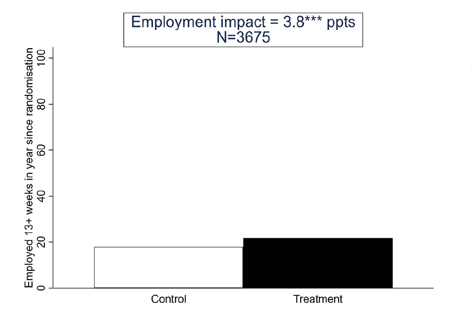
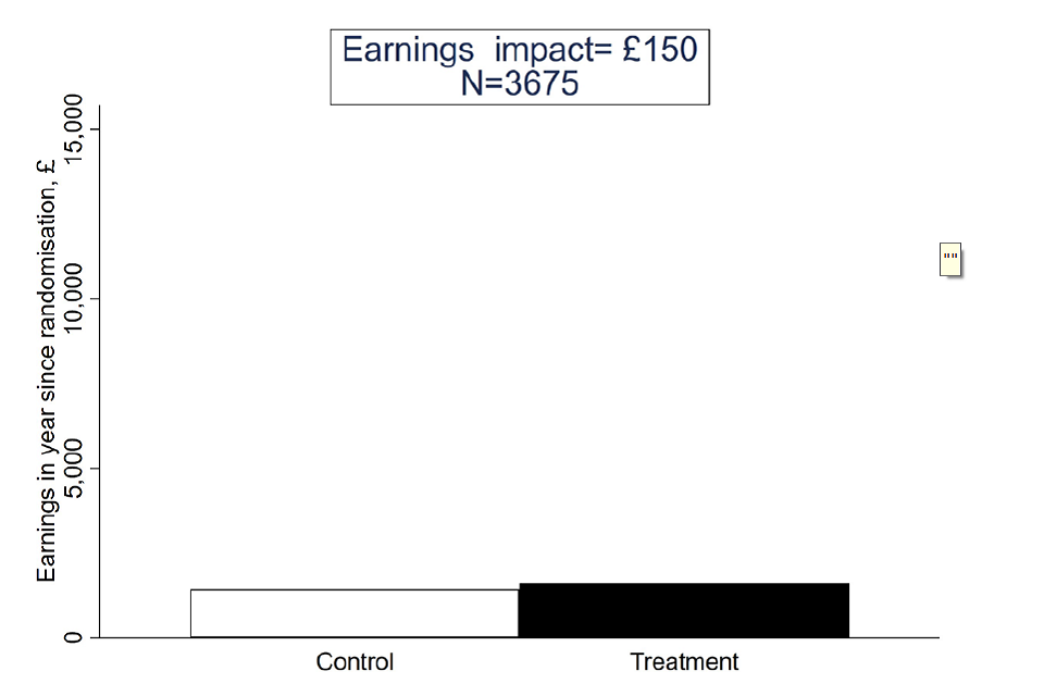
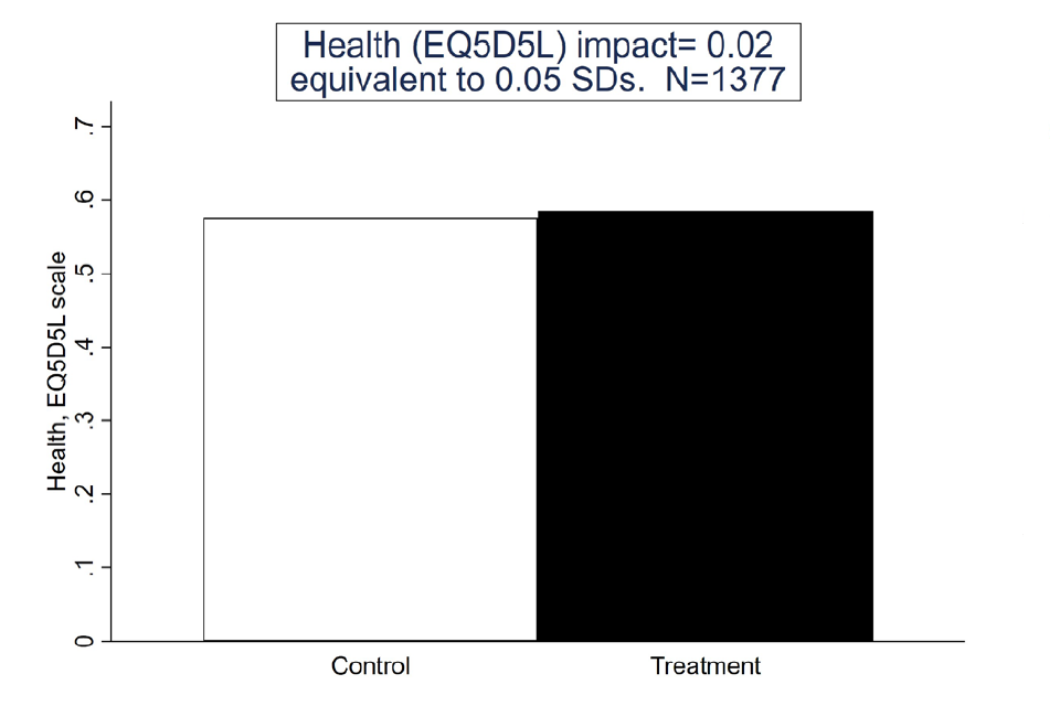
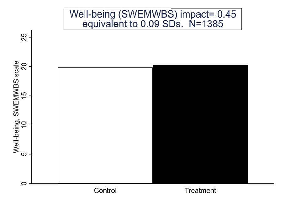
For those in WMCA, there was a substantial positive impact on employment, significant at the 99% confidence level (see Figure 1). The treatment group were nearly 4 percentage points (ppt) more likely to have been in work for 13 or more weeks in the year following randomisation than the control group. Relative to the control group, this represents an increased employment probability of more than 20 per cent. However, there were no significant impacts on earnings, or health and wellbeing outcomes.

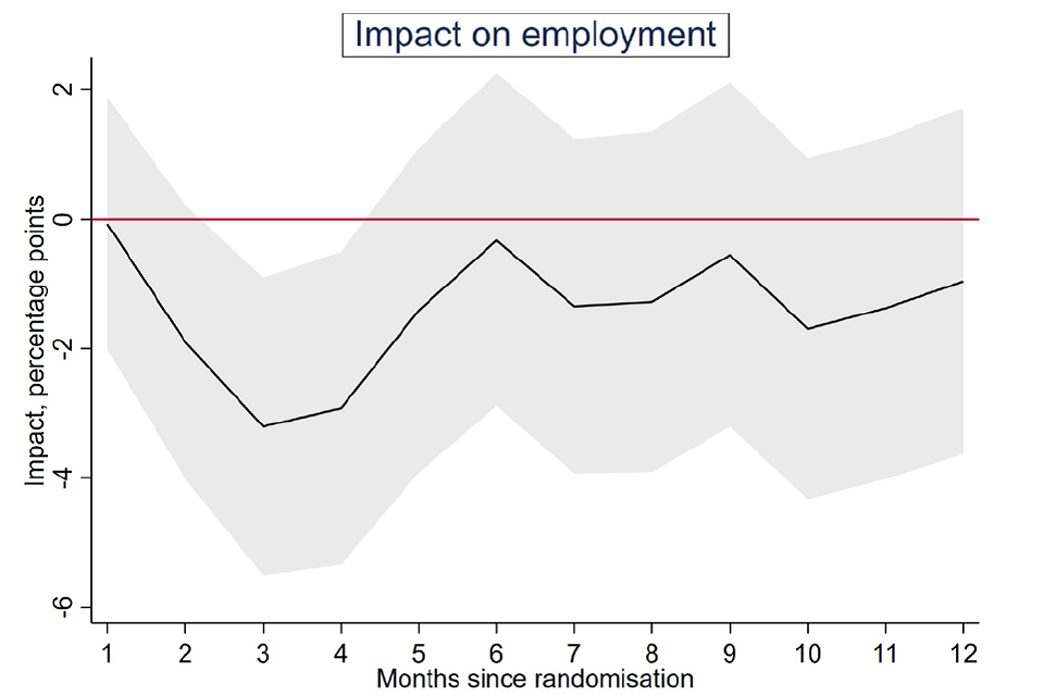
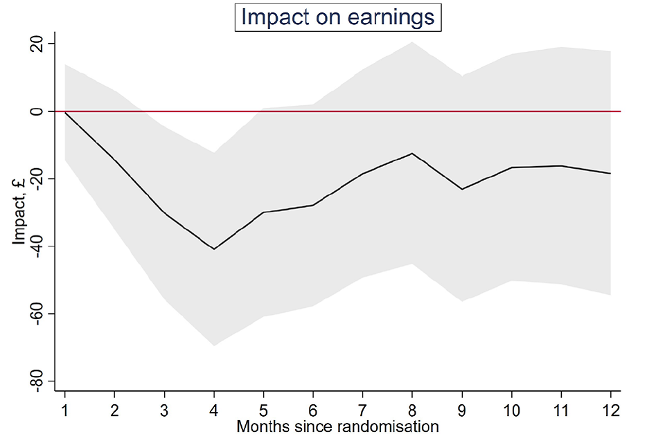
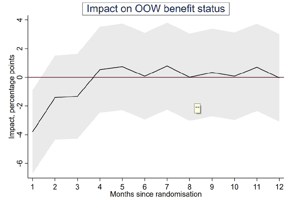
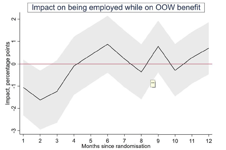
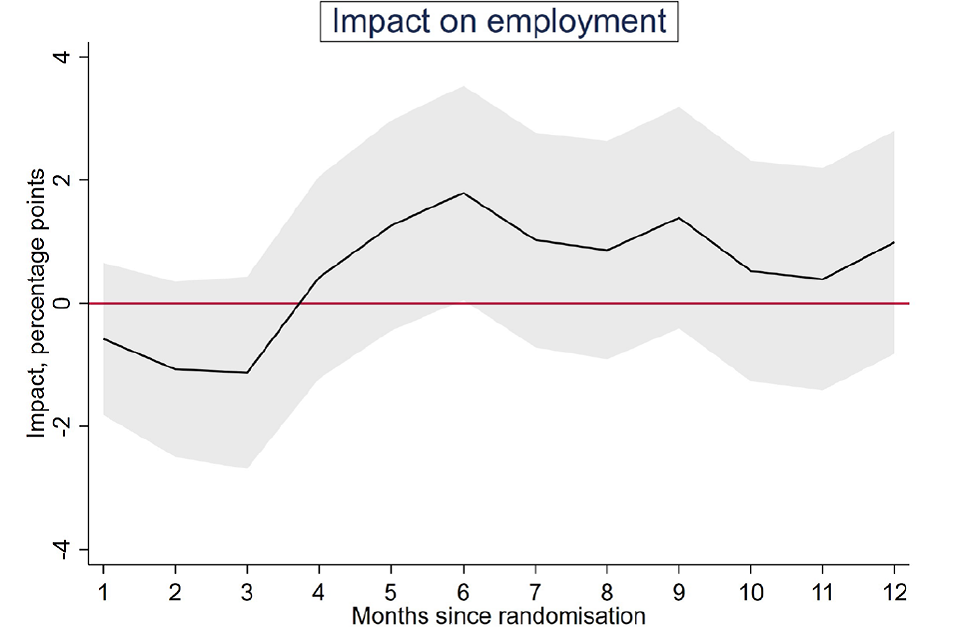
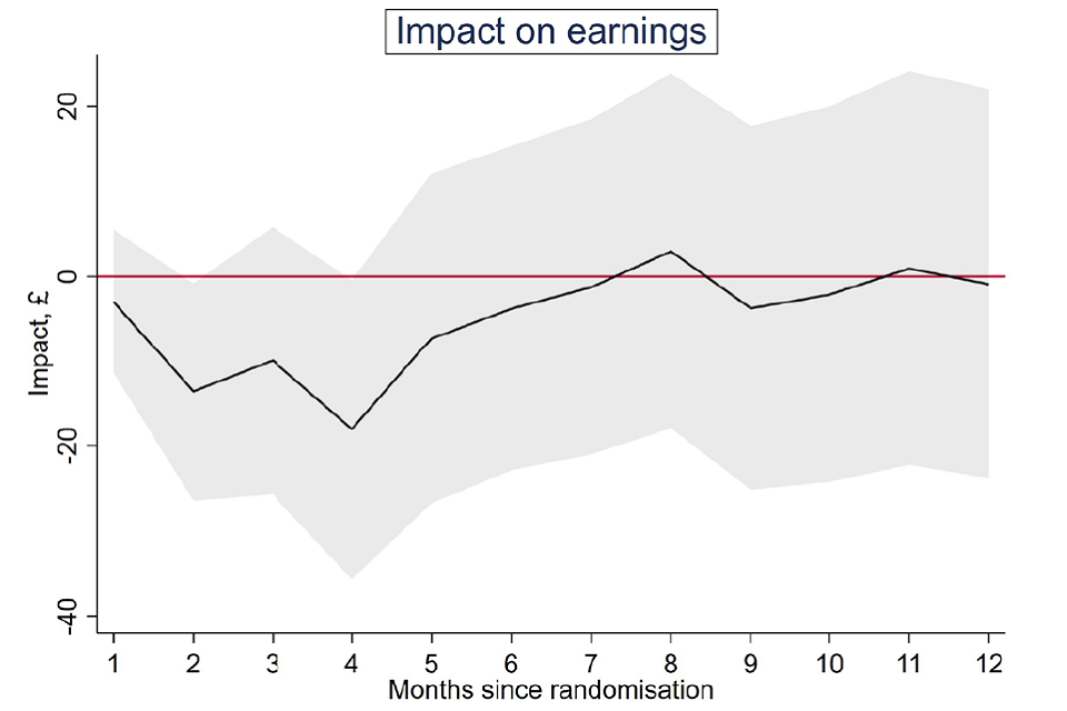
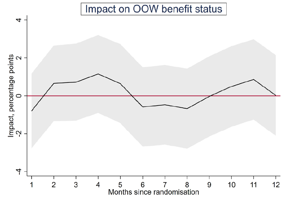
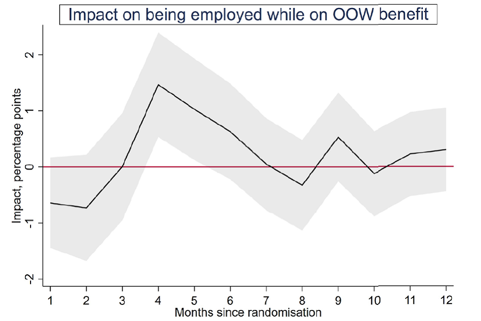
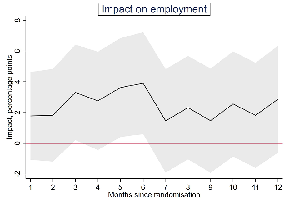
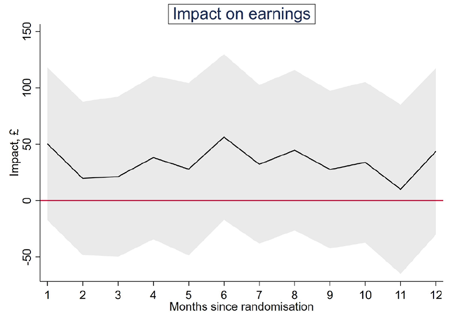
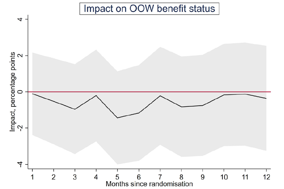
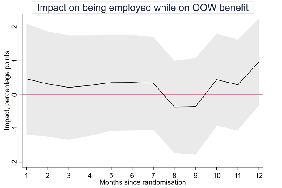
Among the secondary outcomes, the number of months in work was increased by 0.3 (see Table 2.2). No other secondary outcomes showed a significant impact (see Appendix Table A2.7). However, looking at the monthly impacts, from 4 months post-randomisation, the impact on employment is consistently positive and statistically significant. The impact on earnings also reaches a stable positive level but does not achieve statistical significance. The impact on benefit receipt is consistently non-significant while being employed and receiving a welfare benefit is significantly increased during the first 6 months, but there was no increase beyond this. In combination with the monthly results seen for employment, this is suggestive of individuals increasing their employment without initially changing their benefit status, but over time remaining in work without out-of-work benefits.

The subgroup analysis provides little evidence of variation across the groups considered (see Appendix Table A2.8). It is only with wellbeing that some significant variation is found (see Table 2.3), with positive impacts concentrated among individuals whose baseline health was in the middle third.

Figure 1: Primary outcomes for WMCA

Asterisks denote confidence level: 90%, **95%, **99%

Source: Final, linked data set.

Table 2.2: Statistically significant secondary outcomes for WMCA

WMCA	Control	Treatment	Impact	SE	SDs	P-unadj	P-adj	Sig	N
Number of months employed (HMRC)	1.7	2.0	0.3	0.1	0.09	0.01	0.07	*	3675

Source: Final, linked data set

Figure 2: Monthly outcomes for WMCA

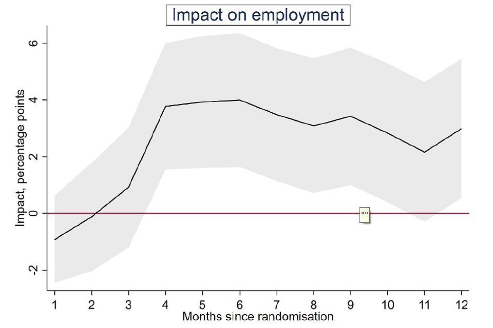
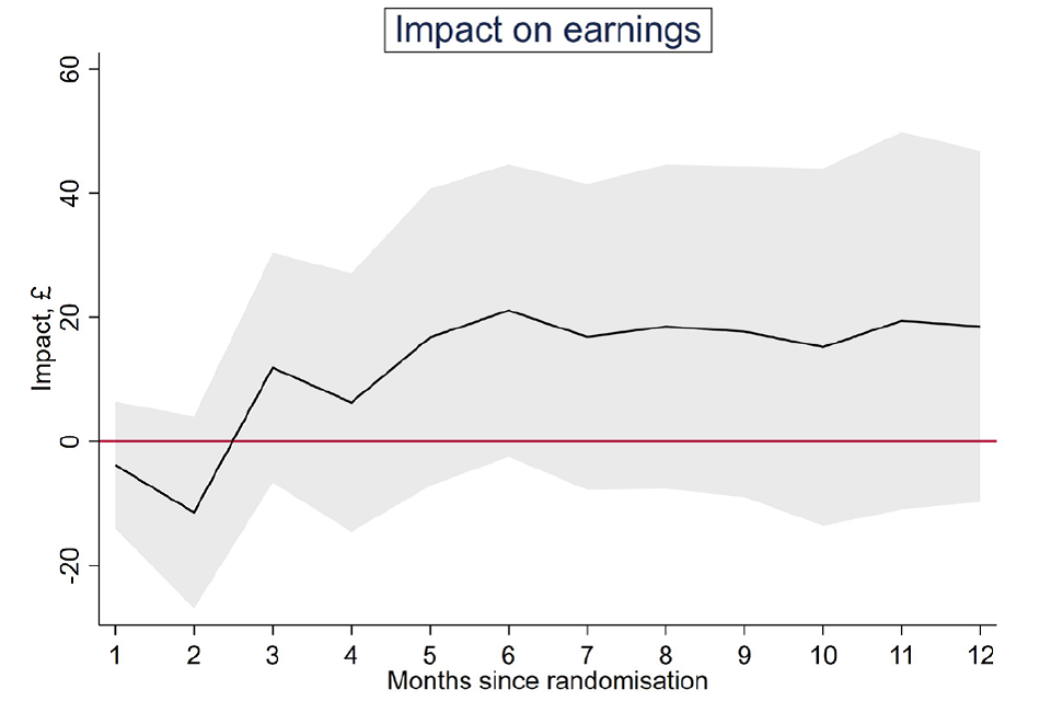
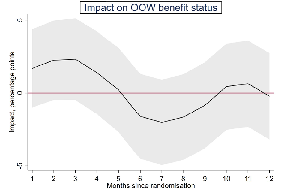
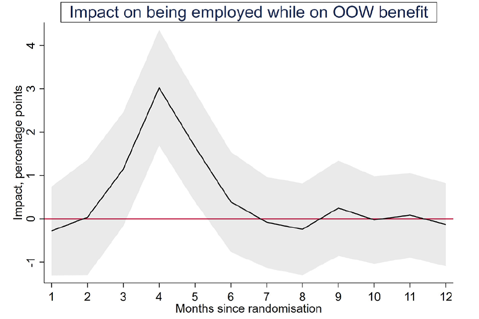
Impacts depicted by solid black line; 95% confidence intervals as grey areas

Source: Final, linked data set.

Table 2.3: Statistically significant subgroup variation among primary outcomes for WMCA

	Employment: impact	Employment: sig.	Earnings: impact	Earnings: sig.	Health: impact	Health: sig.	Wellbeing: impact	Wellbeing: sig.
Health (EQ5D5L)	–	–	–	–	–	–	–	**
Bottom third	0.02	–	115.66	–	0.03	–	0.05	–
Middle third	0.02	–	-106.05	–	0.02	–	1.35	–
Top third	0.07	–	395.58	–	0.00	–	-0.02	–

Asterisks denote confidence level: 90%, **95%, **99%

Source: Final, linked data set.

Table 2.4: Participation impact estimates (WMCA)

	Impact	SE	SDs	P-unadj	P-adj	Sig	N
Employed for 13 or more weeks, % (HMRC)	4.1	1.4	–	0.00	0.01	***	3675
Total earnings, £ (HMRC)	162	125	–	0.20	0.36	–	3675
Health (EQ5D5L) (final survey)	0.02	0.01	0.05	0.22	0.36	–	1377
Wellbeing (SWEMWBS) (final survey)	0.46	0.25	0.09	0.06	0.18	–	1385

Asterisks denote confidence level: 90%, **95%, **99%

Source: Final, linked data set.

2.2.2. Impact estimates for the SCR OOW group

Summary

For the SCR OOW group, being assigned to the treatment group had no statistically significant effect on either employment or earnings (see Figure 3). Positive but small impacts were seen for health and wellbeing (0.10 and 0.12 standard deviations respectively), significant at the 90% confidence level. Among the secondary employment outcomes (see Table 2.5 and Appendix Table A2.3), only job search self-efficacy appeared affected, increasing by 0.13 standard deviations, significant at the 90% confidence level.

Looking at the monthly impacts (see Figure 4), the negative impacts on employment and earnings appear significant at points during the first 6 months post-randomisation (but not beyond). Receipt of out-of-work benefits is also reduced in the month of randomisation.

With regard to health and wellbeing, treatment group individuals were less likely than those in the control group to report musculoskeletal problems or disability more generally. Small positive effects on mental health were found, according to both the GAD survey questions (0.15 standard deviations) and the PHQ survey questions (0.13 standard deviations). Life satisfaction and general self-efficacy were also increased, by 0.13 and 0.12 standard deviations respectively.

Subgroup analysis (see Table 2.6 and Appendix Table A2.4) suggested that earnings impacts varied with age; specifically, that the negative impacts were found among individuals in their thirties and forties. There was no other significant variation in impacts.

Figure 3: Primary outcomes for SCR OOW

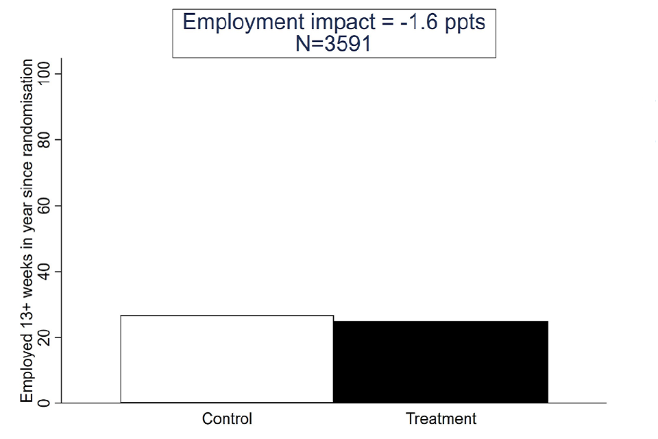
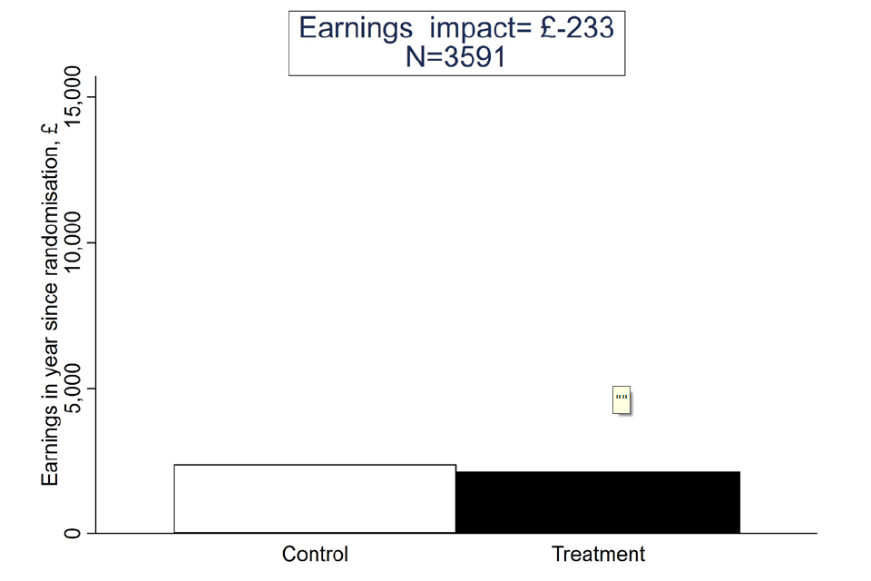
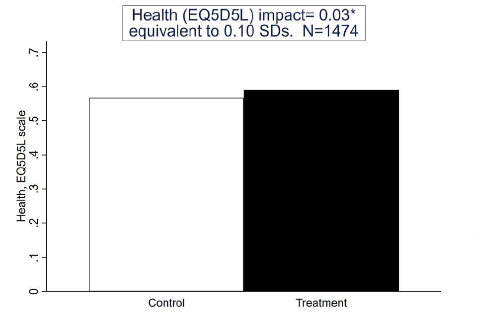
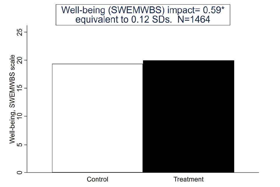
Asterisks denote confidence level: 90%, **95%, **99%

Source: Final, linked data set.

Table 2.5: Statistically significant secondary outcomes for SCR OOW

SCR OOW	Control	Treatment	Impact	SE	SDs	P-unadj	P-adj	Sig	N
Job search self-efficacy	3.1	3.2	0.1	0.0	0.13	0.01	0.05	*	1420
Musculoskeletal problems % (final survey)	31.4	27.2	-4.9	2.1	–	0.02	0.03	**	1492
Disability (DDA definition) % (final survey)	32.2	26.7	-5.6	2.2	–	0.01	0.03	**	1486
Life satisfaction (ONS1) (final survey)	4.9	5.2	0.4	0.1	0.13	0.00	0.01	***	1478
Self-efficacy (GSE) scale (final survey)	26.6	27.5	0.9	0.4	0.12	0.02	0.01	**	1360
Mental health (GAD) (final survey)	9.9	8.9	-1.0	0.3	0.15	0.00	0.00	***	1454
Mental health (PHQ) (final survey)	11.3	10.4	-0.9	0.3	0.13	0.01	0.02	**	1397

Asterisks denote confidence level: 90%, **95%, **99%

Source: Final, linked data set.

Figure 4: Monthly outcomes SCR OOW

Impacts depicted by solid black line; 95% confidence intervals as grey areas

Source: Final, linked data set.

Table 2.6: Statistically significant subgroup variation among primary outcomes SCR OOW

Age	Employment: impact	Employment: sig.	Earnings: impact	Earnings: sig.	Health: impact	Health: sig.	Wellbeing: impact	Wellbeing: sig.
Age	–	–	–	**	–	–	–	–
Under 30	-0.03	–	-155.12	–	0.06	–	0.72	–
30-39	-0.04	–	-634.51	–	0.00	–	0.58	–
40-49	-0.03	–	-666.72	–	0.02	–	0.60	–
50+	0.03	–	200.35	–	0.03	–	0.48	–

Asterisks denote confidence level: 90%, **95%, **99%

Source: Final, linked data set.

Table 2.7: Participation impact estimates (SCR OOW)

Type of participation	Impact	SE	SDs	P-unadj	P-adj		N
Employed for 13 or more weeks, % (HMRC)	-1.8	1.5	–	0.25	0.25	–	3,591
Total earnings, £ (HMRC)	-265	165	–	0.11	0.17	–	3,591
Health (EQ5D5L) (final survey)	0.03	0.01	0.11	0.02	0.05	*	1,474
Wellbeing (SWEMWBS) (final survey)	0.62	0.25	0.12	0.01	0.05	*	1464

Asterisks denote confidence level: 90%, **95%, **99%

Source: Final, linked data set.

2.2.3. All OOW (SCR or WMCA)

Summary

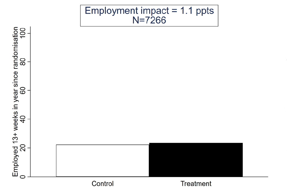
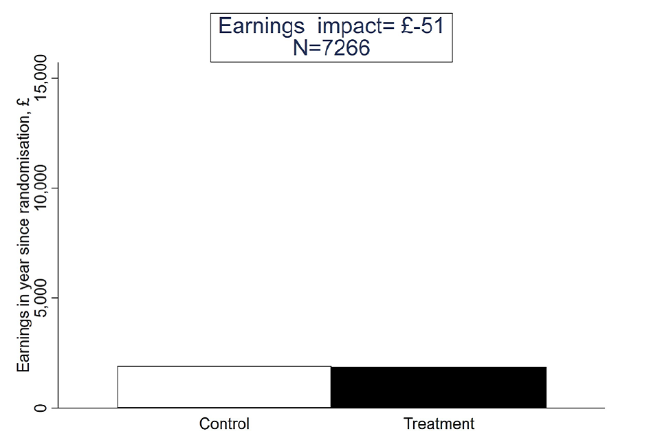
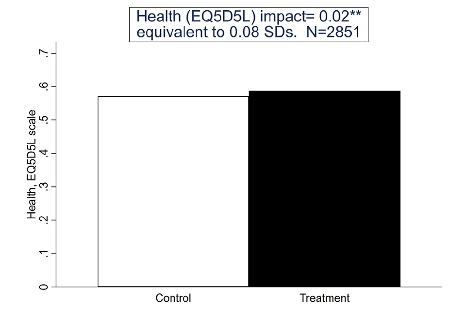
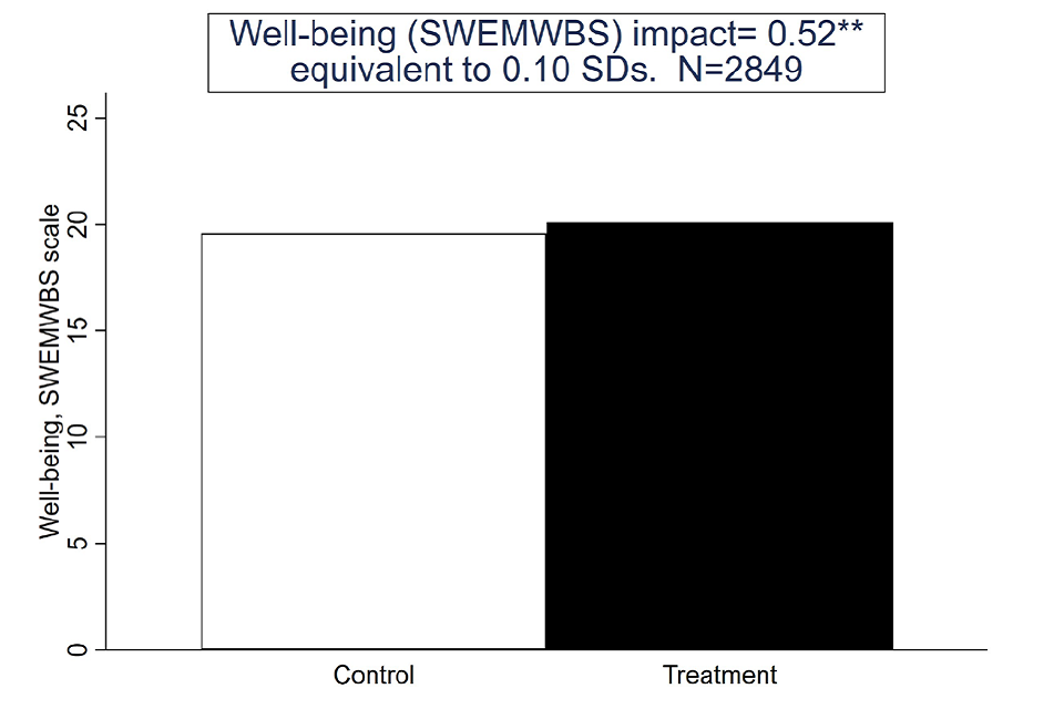
When both OOW groups are pooled, there is no evidence of an employment or earnings effect but the health and wellbeing impacts are both statistically significant (0.08 and 0.10 standard deviations, respectively) at the 95% confidence level (see Figure 5).

Among secondary outcomes (see Table 2.8 and Appendix Table A2.9), there are small positive impacts on job search self-efficacy, mental health and wellbeing. The probability of reporting a musculoskeletal problem was also reduced.

Looking at the monthly impacts, the impression is of no significant impact other than for the probability of being employed while on an out-of-work benefit; this grows to achieve statistical significance in months 4 and 5, mirroring the pattern seen in WMCA (see Figure 6).

Subgroup analysis suggests there may be a greater impact on wellbeing among individuals whose baseline health was in the middle third (see Table 2.9 and Appendix Table A2.10).

Figure 5: Primary outcomes for All OOW

Asterisks denote confidence level: 90%, **95%, **99%

Source: Final, linked data set.

Table 2.8: Statistically significant secondary outcomes for All OOW

All OOW	Control	Treatment	Impact	SE	SDs	P-unadj	P-adj	Sig	N
Job search self-efficacy	3.1	3.2	0.1	0.0	0.09	0.01	0.06	*	2,762
Musculoskeletal problems % (final survey)	29.9	27.8	-3.4	1.5	–	0.02	0.05	*	2,904
Life satisfaction (ONS1) (final survey)	5.1	5.3	0.2	0.1	0.08	0.02	0.03	**	2,883
Self-efficacy (GSE) scale (final survey)	26.9	27.5	0.6	0.3	0.09	0.02	0.03	**	2,625
Mental health (GAD) (final survey)	9.6	8.9	-0.8	0.2	0.12	0.00	0.00	***	2,803
Mental health (PHQ) (final survey)	11.0	10.4	-0.7	0.2	0.10	0.01	0.02	**	2685

Asterisks denote confidence level: 90%, **95%, **99%

Source: Final, linked data set.

Figure 6: Monthly outcomes for All OOW

Impacts depicted by solid black line; 95% confidence intervals as grey areas

Source: Final, linked data set.

Table 2.9: Statistically significant subgroup variation among primary outcomes for All OOW

Subgroup	Employment: impact	Employment: sig.	Earnings: impact	Earnings: sig.	Health: impact	Health: sig.	Wellbeing: impact	Wellbeing: sig.
Health (EQ5D5L)	–	–	–	–	–	–	–	*
Bottom third	0.01	–	38.55	–	0.04	–	0.49	–
Middle third	-0.01	–	-229.61	–	0.02	–	1.03	–
Top third	0.04	–	108.72	–	0.02	–	0.16	–

Asterisks denote confidence level: 90%, **95%, **99%

Source: Final, linked data set.

Table 2.10: Participation impact estimates (All OOW)

Type of participation	Impact	SE	SDs	P-unadj	P-adj		N
Employed for 13 or more weeks, % (HMRC)	1.2	1.0	–	0.24	0.36	–	7,266
Total earnings, £ (HMRC)	-56	103	–	0.59	0.58	–	7,266
Health (EQ5D5L) (final survey)	0.02	0.01	0.08	0.01	0.03	**	2,851
Wellbeing (SWEMWBS) (final survey)	0.54	0.18	0.10	0.00	0.01	***	2,849

Asterisks denote confidence level: 90%, **95%, **99%

Source: Final, linked data set.

2.2.4. Impact estimates for the SCR IW group

Summary

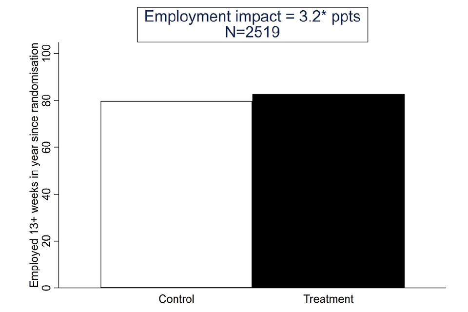
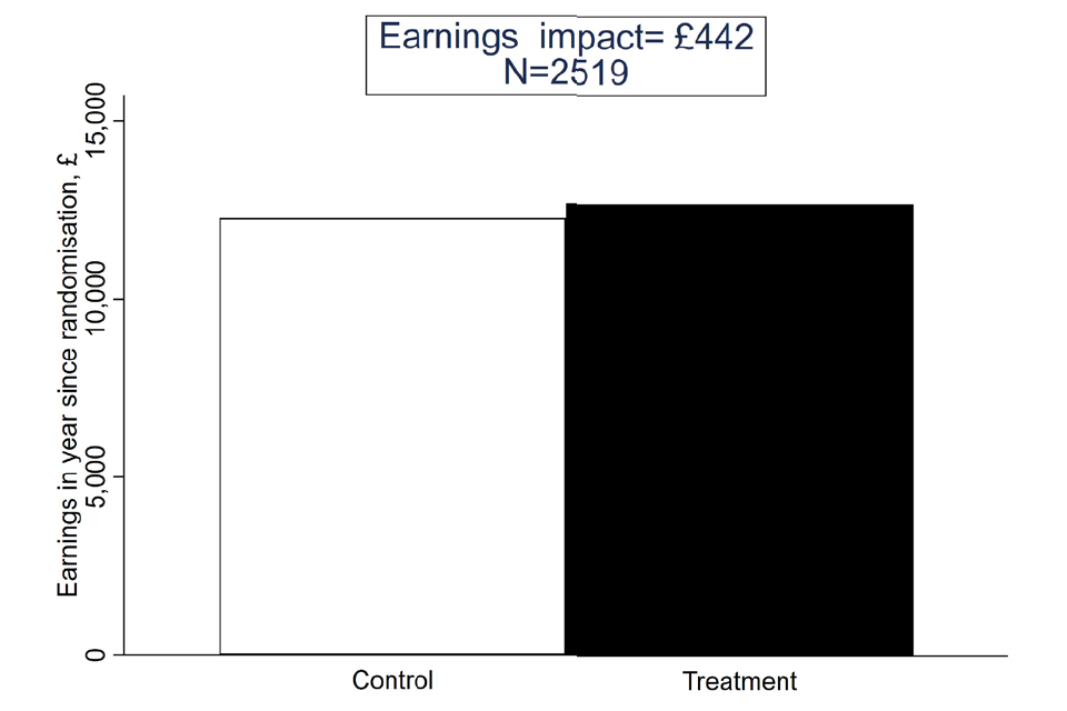
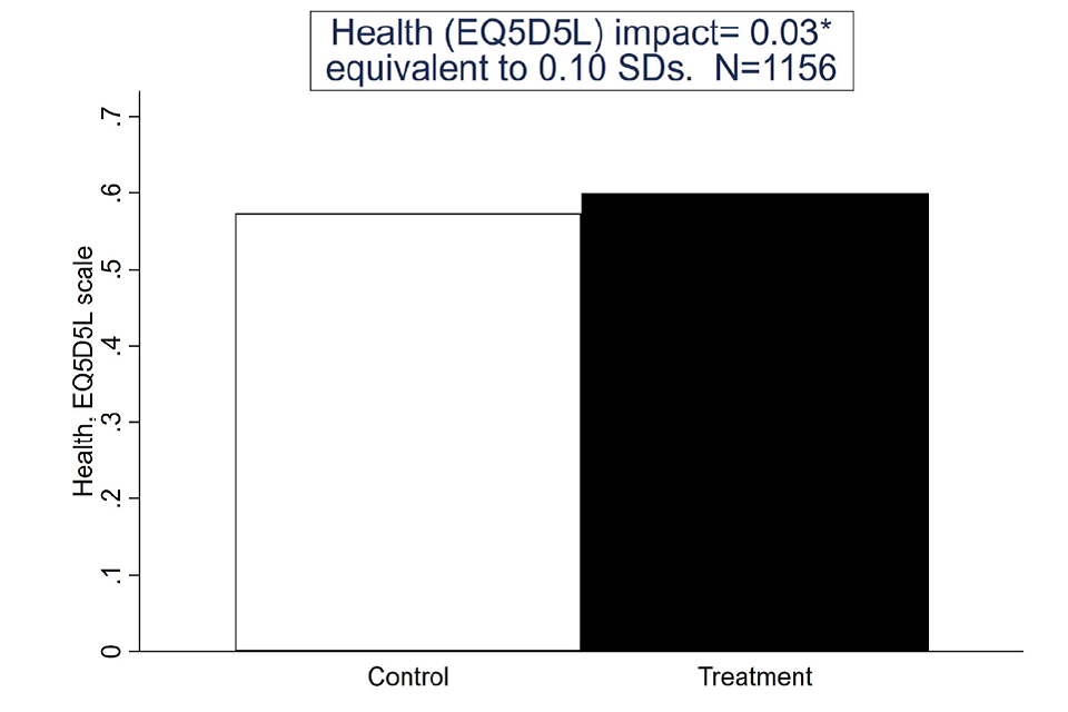
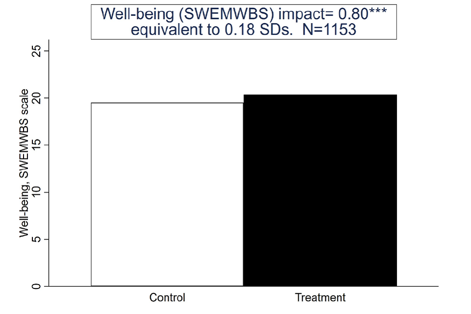
For the SCR IW group, being assigned to the treatment group increased the probability of having been in work for 13 or more weeks in the year following randomisation by 3 percentage points (see Figure 7). This impact is significant at the 90% confidence level. The effect on earnings for the SCR IW treatment group was not statistically significant. There was a small positive impact on health (0.10 standard deviations) that was significant at the 90% confidence level. Impact on wellbeing was both more substantial (0.18 standard deviations) and significant at the 99% confidence level.

Among the secondary outcomes (see Table 2.11 for statistically significant results and Appendix Table A2.1 for all results), there was no evidence of an impact on employment-related outcomes except for job search self-efficacy which was increased by 0.23 standard deviations. In the health domain, the probability of reporting a musculoskeletal problem was reduced by 7 percentage points (ppts). For wellbeing, both life satisfaction and general self-efficacy were significantly increased (0.14 and 0.15 standard deviations, respectively).

Looking at the monthly impacts (see Figure 8), the impact on employment is consistently positive and sometimes achieved conventional levels of statistical significance during the first 6 months post-randomisation. The other outcomes – earnings, benefits and employment while on benefits – do not appear significant in any month.

Subgroup analysis (see Table 2.12 and Appendix Table A2.2) suggested significant variation in the impact on health depending on health at randomisation, with stronger impacts seen for those with lower initial health. Other than this, there is no evidence of statistically significant variation across the dimensions considered.

Figure 7: Primary outcomes for the SCR IW group

Asterisks denote confidence level: 90%, **95%, **99%

Source: Final, linked data set.

Table 2.11: Statistically significant secondary outcomes for the SCR IW group

SCR IW	Control	Treatment	Impact	SE	SDs	P-unadj	P-adj		N
Job search self-efficacy	3.2	3.4	0.3	0.1	0.23	0.00	0.00	***	1,120
Musculoskeletal problems % (final survey)	35.6	29.3	-7.1	2.4	–	0.00	0.01	**	1,166
Life satisfaction (ONS1) (final survey)	5.2	5.7	0.4	0.1	0.14	0.01	0.02	**	1,155
Self-efficacy (GSE) scale (final survey)	27.6	28.6	0.9	0.4	0.15	0.01	0.02	**	1,111

Asterisks denote confidence level: 90%, **95%, **99%

Source: Final, linked data set.

Figure 8: Monthly outcomes SCR IW

Impacts depicted by solid black line; 95% confidence intervals as grey areas

Source: Final, linked data set.

Table 2.12: Statistically significant subgroup variation among primary outcomes SCR IW

Subgroup	Employment: impact	Employment: sig.	Earnings: impact	Earnings: sig.	Health: impact	Health: sig.	Wellbeing: impact	Wellbeing: sig.
Health (EQ5D5L)	–	–	–	–	–	**	–	–
Bottom third	0.03	–	213.30	–	0.07	–	1.21	–
Middle third	0.03	–	423.89	–	0.04	–	1.02	–
Top third	0.03	–	899.57	–	-0.02	–	0.05	–

Asterisks denote confidence level: 90%, **95%, **99%

Source: Final, linked data set.

Table 2.13 : Participation impact estimates (SCR IW)

SCR IW	Impact	SE	SDs	P-unadj	P-adj		N
Employed for 13 or more weeks, % (HMRC)	3.5	1.6	–	0.03	0.10	*	2,519
Total earnings, £ (HMRC)	484	391	–	0.22	0.22	–	2,519
Health (EQ5D5L) (final survey)	0.03	0.01	0.11	0.04	0.10	*	1,156
Wellbeing (SWEMWBS) (final survey)	0.82	0.26	0.19	0.00	0.01	***	1,153

Asterisks denote confidence level: 90%, **95%, **99%

Source: Final, linked data set.

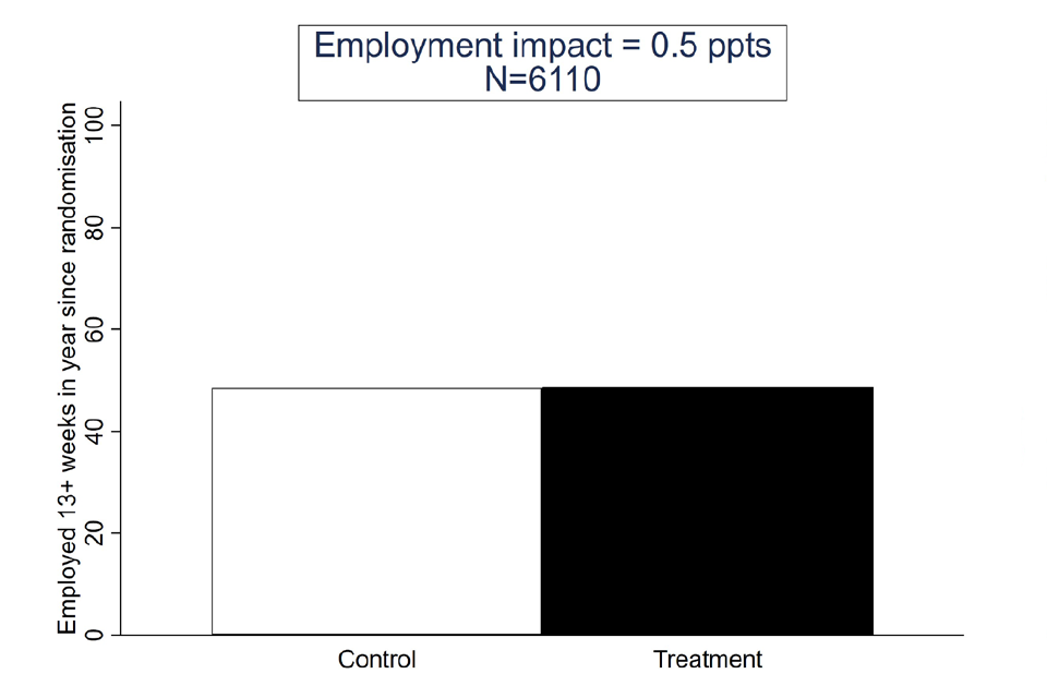
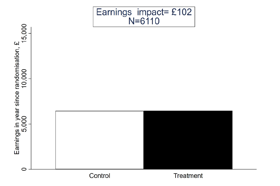
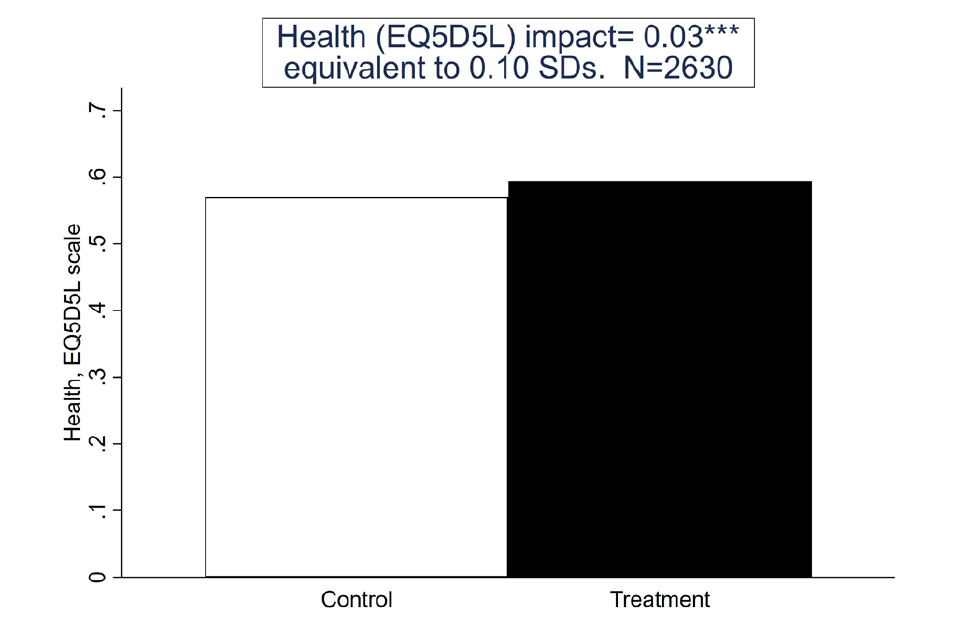
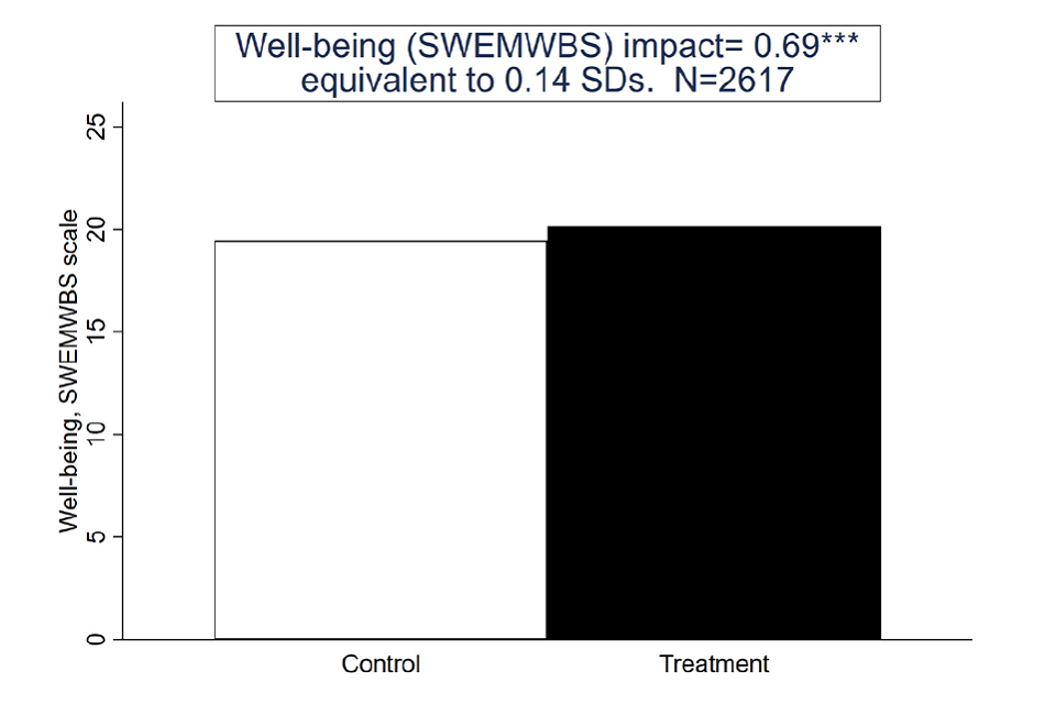
2.2.5. Impact estimates for All SCR (IW or OOW)

Summary

The results in this section relate to SCR as a whole, regardless of employment status at the time of randomisation (see Figure 9). They are similar to the separate IW and OOW results in finding no effect on employment or earnings but stronger positive impacts on health and wellbeing. Among the primary outcomes, the impacts on health and wellbeing are significant at the 99% confidence level, despite being small (0.10 and 0.14 standard deviations, respectively).

Among the secondary outcomes (see Table 2.14 and Appendix Table A2.5), there was a small significant positive impact on job search self-efficacy (0.18 standard deviations) but no other employment outcomes. Health and wellbeing impacts were statistically significant. Both measures of mental health showed improvement due to being allocated to the treatment group of 0.11 standard deviations. Musculoskeletal problems were reduced by 6 ppt and the extent to which disability was reported by the treatment group reduced by 4 ppt. In respect of wellbeing, both life satisfaction and general self-efficacy were improved, by 0.14 standard deviations. Looking at the monthly impacts (see Figure 10) suggests a reduction in benefit receipt in the month of randomisation but no significant impacts beyond that or for any of the other outcomes.

Subgroup analysis did not provide any evidence of statistically significant variation across the dimensions considered (see Appendix Table A2.6).

Figure 9: Primary outcomes SCR

Asterisks denote confidence level: 90%, **95%, **99%

Source: Final, linked data set.

Table 2.14: Statistically significant secondary outcomes for All SCR

All SCR	Control	Treatment	Impact	SE	SDs	P-unadj	P-adj	Sig	N
Job search self-efficacy	3.1	3.3	0.2	0.0	0.18	0.00	0.00	***	2,540
Musculoskeletal problems % (final survey)	33.1	28.1	-5.8	1.6	–	0.00	0.00	***	2,658
Disability (DDA definition) % (final survey)	30.3	26.1	-4.2	1.7	–	0.01	0.01	**	2,641
Life satisfaction (ONS1) (final survey)	5.1	5.4	0.4	0.1	0.14	0.00	0.00	***	2,633
Self-efficacy (GSE) scale (final survey)	27.0	28.0	0.9	0.3	0.14	0.00	0.00	***	2,471
Mental health (GAD) (final survey)	9.7	9.0	-0.7	0.2	0.11	0.00	0.01	***	2,598
Mental health (PHQ) (final survey)	11.2	10.4	-0.8	0.3	0.11	0.00	0.01	***	2,516

Asterisks denote confidence level: 90%, **95%, **99%

Source: Final, linked data set.

Figure 10: Monthly outcomes All SCR

Impacts depicted by solid black line; 95% confidence intervals as grey areas Source: Final, linked data set.

Table 2.15: Participation impact estimates (All SCR)

Type of participation	Impact	SE	SDs	P-unadj	P-adj	Sig	N
Employed for 13 or more weeks, % (HMRC)	0.6	1.2	–	0.61	0.79	–	6,110
Total earnings, £ (HMRC)	114	205	–	0.58	0.79	–	6,110
Health (EQ5D5L) (final survey)	0.03	0.01	0.10	0.00	0.01	***	2,630
Wellbeing (SWEMWBS) (final survey)	0.72	0.18	0.15	0.00	0.00	***	2,617

Asterisks denote confidence level: 90%, **95%, **99%

Source: Final, linked data set.

2.3. Discussion

The results in this report focus on outcomes observed for trial recruits in the 12 months following randomisation. They therefore can be viewed as covering a period of time over which one might reasonably expect the impacts of IPS to be visible, if it is effective (although, this is not guaranteed). This reflects the intuition not only that individuals’ outcomes take time to respond to IPS – the literature suggests that employment impacts of IPS, for example, take 4 to 6 months to materialise – but also that the nature of the IPS service itself matured after the initial launch of the trial. As evidence of this last point, the reviews of IPS fidelity, as is typical for IPS services, suggested that it took some time for the treatment to be delivered in line with IPS principles in WMCA (in SCR, there was no information on how quickly fidelity was achieved).

In considering the results, we focus first on individuals who were out of work (OOW) at the time of randomisation. IPS significantly increased sustained employment (that is, employment of 13 or more weeks) but not health or wellbeing in WMCA. By contrast, IPS significantly increased health and wellbeing but not sustained employment for SCR OOW. In both cases, there was no effect on earnings. A key question is why there should be such a difference between the sites. For the health and wellbeing outcomes, it is possible that this reflects differences between the sites in the support provided. Qualitative evidence (contained in the implementation and 4-month outcomes and the CMO reports) suggests that SCR emphasised health outcomes more than WMCA, which in turn was more focused on employment.

Differences in how the support was delivered may have played a role. The results on IPS engagement show how the proportion of the treatment group receiving any sort of IPS support was greater in WMCA than in SCR and this was also true when considering more detailed support (a session lasting more than 15 minutes). Eligible individuals began their IPS support more quickly in WMCA and there was a greater use of follow-up calls.

Another possibility is that IPS may be more effective for some people than others and that compositional differences between the WMCA and SCR OOW groups would lead us to expect bigger impacts in WMCA. We probed this for the employment outcome by pooling SCR OOW with WMCA and then estimating impacts, allowing these to vary with observed characteristics. Were compositional differences alone sufficient to explain the difference in impacts between the two areas, we would expect there to be no remaining difference once such variations were controlled for. Instead, a difference remained, suggesting that compositional differences did not explain the variation in impacts.

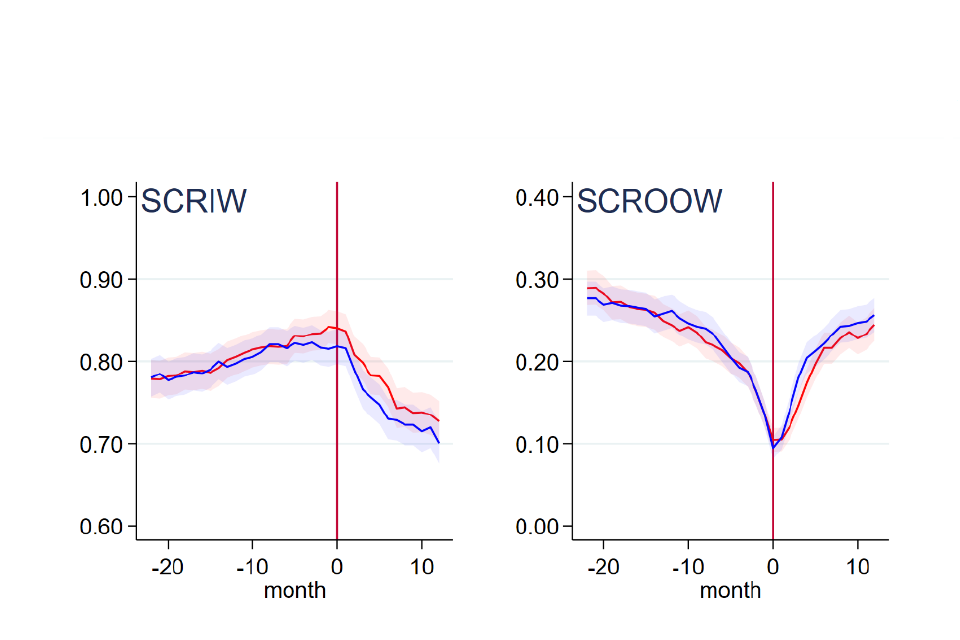
Figure 11 looks deeper, charting monthly employment and the earnings for treatment and control groups. Comparing the control groups for SCR OOW and WMCA reveals two potentially relevant differences. First, the employment rate is generally higher in SCR than in WMCA. This could indicate greater employability among the SCR OOW group or reflect the fact that the local labour market in SCR offers more employment opportunities than WMCA (see the labour market analysis contained in the report entitled ‘The pandemic and the trials’). While there is no basis for thinking that compositional differences explain the stronger performance of IPS in WMCA, it may be that the nature of the labour market is important and that there is a greater role for IPS in more depressed labour markets.

Second, control group individuals in SCR tend to have more success than those in WMCA when re-entering employment. In SCR, the control group employment rate 12 months prior to randomisation was 26% and 12 months post-randomisation it was back at that level. In WMCA, by contrast, the control group employment rate 12 months prior to randomisation was 22% and 12 months post-randomisation had only recovered to 18%. As when considering the impact of IPS, control group outcomes may be affected by the composition of the population, the strength of the labour market or the nature of the support available. We explored this by examining the difference in the employment outcome after controlling for the influence of observed characteristics. The difference between SCR OOW and WMCA remained substantial. This adds weight to the belief that it is driven either by different labour markets or by more support being available to the control group in SCR.

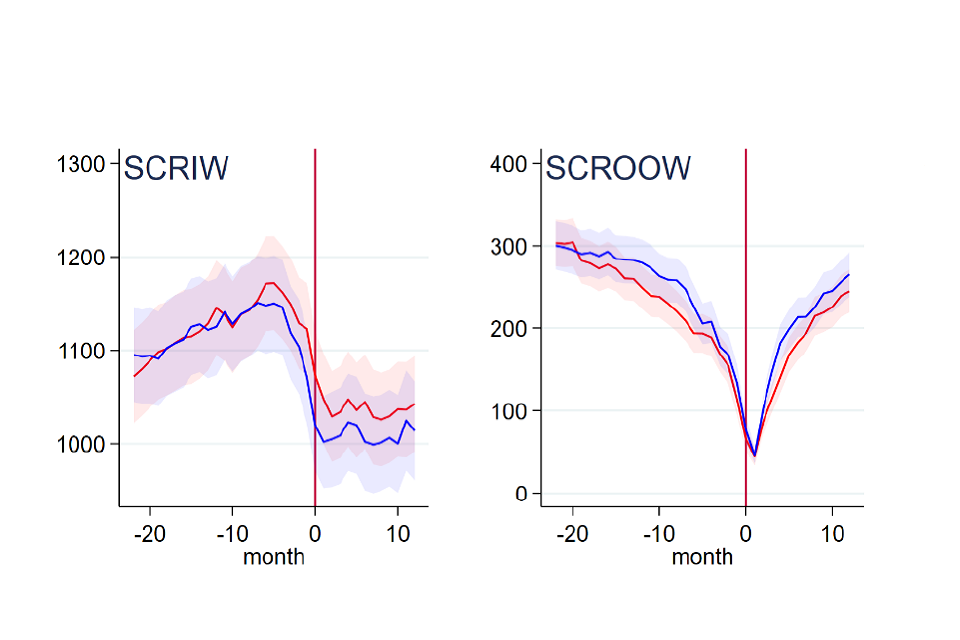
Figure 11: Employment (top row) and earnings (bottom row) by month for treatment (red) and control (blue) groups, shown with 95% confidence intervals

Source: Final, linked data set

Turning to the IW group in SCR, survey respondents had higher levels of employment pre-randomisation than trial recruits as a whole and this remained the case after weighting. This raises a concern about the representativeness of the survey-based impact estimates for this group. The fact that it was an issue that affected the treatment group more than the control group raises a further concern about whether SCR IW impacts for survey outcomes can be regarded as causal. This is allayed to some extent by the consistency of the estimated impacts on survey-based primary outcomes – health and wellbeing – with those seen for SCR OOW (where there is no such concern regarding the reliability of the weights). With regard to sustained employment, there is some evidence of a positive impact. From Figure 11, it is apparent that employment rates fell quite sharply among the control group. This is perhaps suggestive of there being little support available for those in work, relative to those out of work. If so, there may be a greater role for IPS.

As a final comment, we consider whether for more recent trial entrants outcomes were influenced by COVID-19. To probe this, the subgroup analysis was extended beyond that in the SAP to consider three separate cohorts: an early cohort whose 12-month outcomes pre-dated the pandemic; a middle cohort whose 12-month outcomes fell after the onset of the pandemic but whose experience of IPS is likely to pre-date the pandemic; and a late cohort for whom both the IPS treatment and their outcomes will have been affected by the pandemic. The results of the subgroup analysis did not provide any evidence of impacts varying across these subgroups.

Appendices

A1 Description of the trial populations

The trials recruited between 8 May 2018 and 31 October 2019. Over this time, 9,785 individuals were randomised. Figure A1.1 shows the numbers recruited each month, by trial group. After initial growth through to autumn 2018, intake remained fairly steady, growing gently in later months before peaking sharply in the final month, October 2019, which accounted for 16% (1,597) of all recruits. This was more than double the number randomised in any other month.

The number of out-of-work (OOW) recruits in any month was quite similar in Sheffield City Region (SCR) and West Midlands Combined Authority (WMCA), while the number in work (IW) in SCR was consistently lower.

Figure A1 Recruitment to trials by month

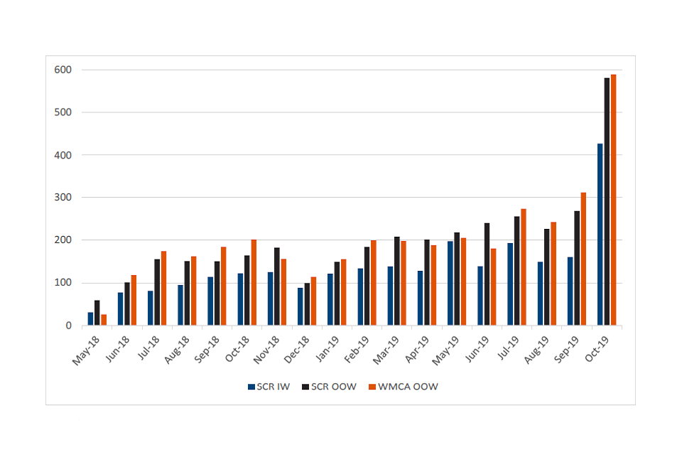
Source: Randomisation tool, all recruits

Table A1.1 shows that, of the 9,785 individuals randomised, 4,896 were assigned to the treatment group and 4,889 were assigned to the control group. Among recruits as a whole, this 50/50 split was visible within all trial groups: SCR IW, SCR OOW and WMCA.

Balance between trial arms (that is, treatment and control groups) is to be expected since it was hard-wired into the software used to conduct the allocation (the randomisation tool).

However, this was not the case among the survey respondent sample. A total of 4,087 individuals were interviewed in the 12-month survey, covering 42% of all those recruited to the trials. Care was taken to ensure that the same survey approach was used for treatment and control groups. For instance, while it would have been possible to update contact details of the treatment group using records from IPS providers, this was avoided so as not to introduce a systematic difference between treatment and control groups.

Despite such precautions, it is clear from Table A1.1 that there was a higher tendency among the treatment group to respond to the survey.

Table A1.1: Numbers randomised and surveyed at 12 months

Survey	SCR: IW (T)	SCR: IW (C)	SCR: OOW (T)	SCR: OOW (C)	WMCA (T)	WMCA (C)	All sites (T)	All sites (C)	All sites (All)
Total randomised	1,260	1,259	1,799	1,792	1,837	1,838	4,896	4,889	9,785
Final survey respondents	631	535	771	732	754	664	2,156	1,931	4,087
Respondent %	50.1	42.5	42.9	40.8	41.0	36.1	44.0	39.5	41.8

Source: Baseline and final survey, all recruits

The difference in response rates could affect whether these data provide unbiased estimates of impact on outcomes drawn from survey data. For this reason, it is appropriate to consider the extent to which the treatment and control groups look similar in respect of observed characteristics. Tables A1.1 to A1.3 summarise the baseline characteristics for the three trial groups. In each case, this is shown separately for the full population, the respondent sample, and the respondent sample broken down by control and treatment group. All characteristics (with the exception of age) are shown as proportions.

While some differences would be expected between the treatment and control groups, if randomisation has been effective, these should not be substantial. To investigate the differences, we conducted statistical tests of similarity among respondents. The results of these tests are summarised using p-values, shown in the final column of each table. For each variable, the p-value indicates how likely it is that the observed treatment-control difference seen among respondents would arise by chance rather than reflecting a true underlying difference. A small p-value suggests the observed difference is unlikely to have arisen by chance and therefore gives grounds for thinking that the difference is statistically significant. If this were the case, this difference in the characteristics of the treatment and control groups might account for differences in outcomes, rather than the treatment – that is, the IPS support. Conventionally, p-values of less than 0.05 are interpreted as being significant in a statistical sense. However, this is essentially arbitrary and cannot be taken to imply that p-values of 0.06, for example, should be ignored.

The results of these analyses (see Tables A1.1 to A1.3) show that those from white ethnic backgrounds are consistently over-represented in the respondent treatment group. The only other significant difference related to health conditions in the SCR OOW group. However, when conducting multiple comparisons, a small proportion would be expected to register as statistically significant purely by chance. With this in mind, the baseline characteristics considered look quite similar across treatment and control groups in the respondent samples.

The concern about treatment-control imbalance prompted the decision rule in the Statistical Analysis Plan (SAP)^{[footnote 8]}:

If there is a treatment-control difference in the response rate of more than 5 percentage points and if baseline measures of job search efficacy, employment history, health or wellbeing differ significantly (p-value <0.05 after adjusting for multiple testing using Westfall-Young (1993)) in weighted regressions on the control variables then regard as primary outcomes sustained employment and earnings taken from the administrative data, and all other outcomes as secondary.

The implication of this decision rule is that if the criteria suggest the survey data may be unreliable for the purpose of impact evaluation, the two primary outcomes that are being measured through survey data – health and wellbeing – would be demoted to secondary outcomes. In this scenario, the primary focus of the evaluation would shift to those outcomes that are observed in administrative data.

The treatment-control difference in response rates is presented in Table A1.2 below. Across all sites, the treatment-control difference is less than 5 percentage points, so the decision rule implies that the choice of primary outcomes remains valid.

Table A1.2: Treatment-control differences in response rates, by site

Group	Treatment group response rate (%)	Control group response rate (%)	Treatment-control difference (ppts)
SCR IW	50.1	42.5	7.6
SCR OOW	42.9	40.8	2.0
WMCA OOW	41.0	36.1	4.9
All sites	44.7	39.8	4.8

Source: Final survey

However, this is rather marginal and at the site level is not satisfied in SCR IW. In view of this, the second criterion of the decision rule – the test of baseline differences – was also conducted. The results are reported in Table A1.3 for baseline outcomes for employment (proxied by ‘looking for work’, ‘job search self-efficacy’ and ‘number of barriers to work’), health (EuroQol-5D-5L, or ‘EQ5D5L’) and wellbeing (Short Warwick-Edinburgh Mental Wellbeing Scale, or ‘SWEMWBS’). In each case, the result shown is p-value of the significance of the baseline difference, after controlling for multiple testing. It is clear that none of the differences is statistically significan ^{[footnote 9]}. Accordingly, based on this element of the decision rule, the primary outcomes remain valid.

Table A1.3: Treatment-control differences in baseline outcomes; p-values of significance tests

Employment status	SCR IW	SCR OOW	WMCA OOW
Looking for work	0.85	0.56	0.82
Job search self-efficacy	0.96	0.39	0.82
Number of barriers	0.96	0.39	0.82
EQ5D5L	0.96	0.56	0.62
SWEMWBS	0.96	0.91	0.49

Source: Baseline and final survey, all respondents

It is nevertheless apparent that a) the 12-month survey respondent sample accounts for less than half of all trial participants and b) the proportion represented is higher among the treatment group than the control group.

Figure A2: Employment rate among 12-month survey respondents and non-respondents

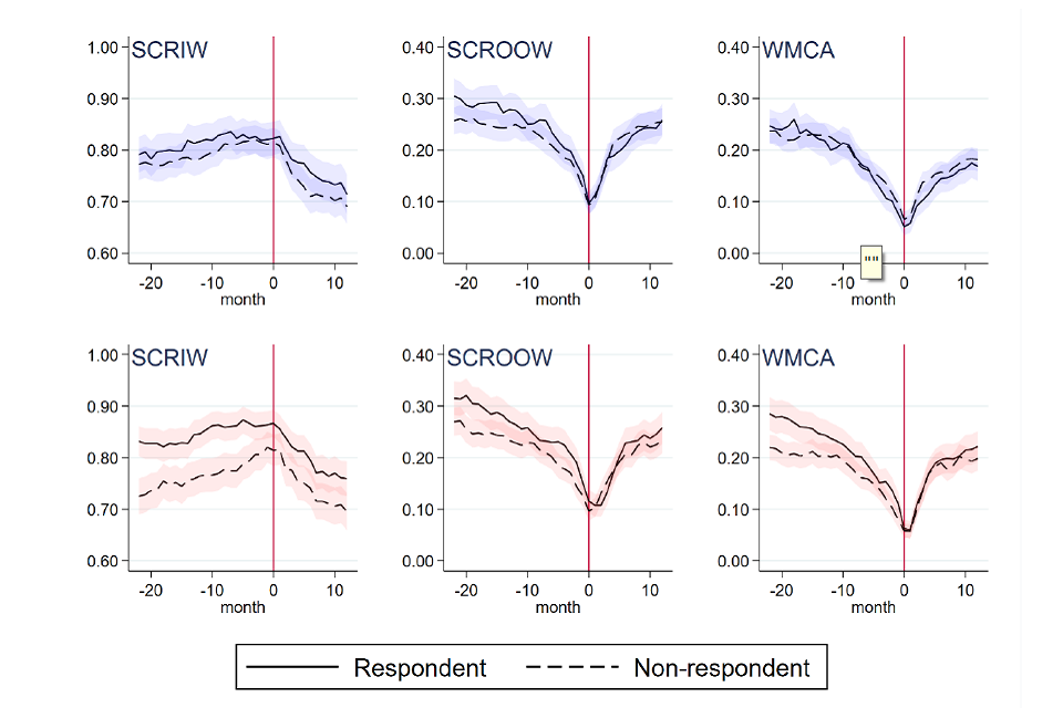
Note: The top row shows the employment history for the control group; the bottom row shows the employment history for the treatment group.

Source: Linked HMRC data

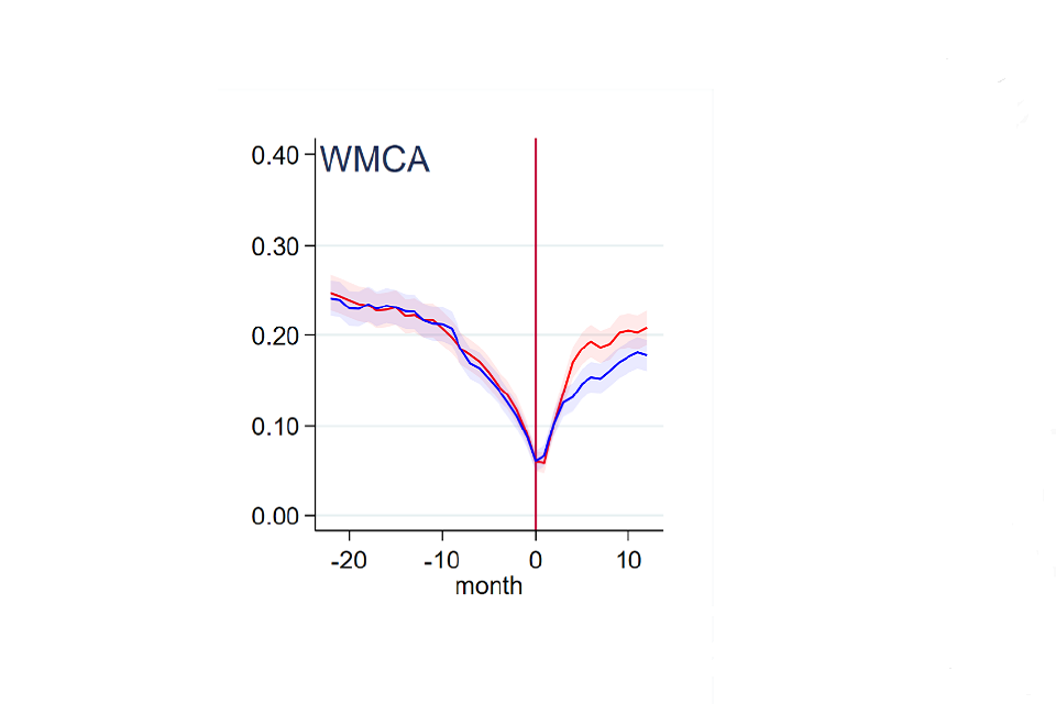
Figure A2 uses linked HMRC data to plot the monthly employment rate over the 2 years preceding randomisation (shown by the vertical line at month 0) for respondents and non-respondents. These look reasonably similar for SCR IW, SCR OOW and WMCA control groups, as evidenced by the confidence intervals (blue shading surrounding both trend lines) overlapping in the pre-randomisation period. For the treatment groups (bottom row) it is apparent that respondents are more likely than non-respondents to be in work in any month prior to randomisation. This difference is statistically significant in the case of SCR IW.

Figure A3: Employment rates for the weighted 12-month respondent sample and the trial population

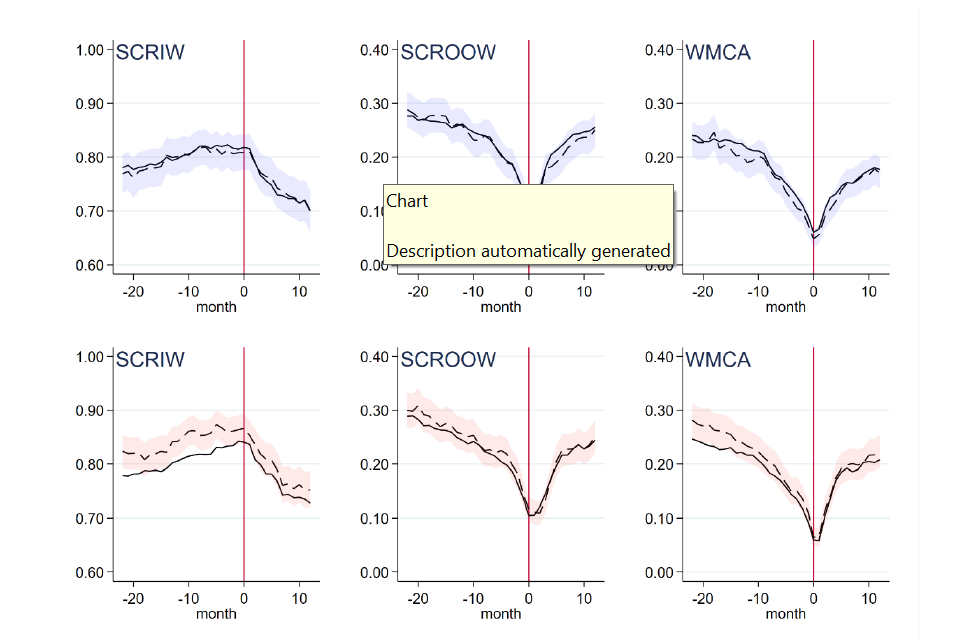
Note: The top row shows the employment history for the control group; the bottom row shows the employment history for the treatment group. Dashed lines cover respondents; population shown with solid lines.

Source: Linked HMRC data

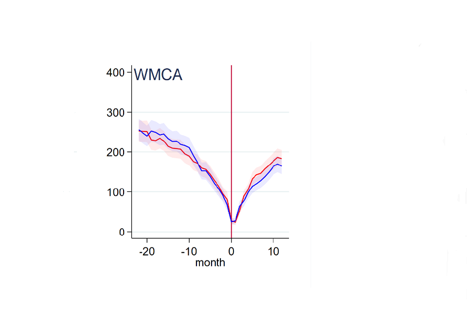
Estimates using the respondent sample are weighted in an attempt to address the possible biasing effect of such imbalance. Figure A3 illustrates the effectiveness of weighting by comparing the employment rate (using linked HMRC data) among survey respondents after applying weights (dashed lines, shown with confidence intervals) with that among the trial population as a whole (solid lines). Again, the top row covers the control group and shows survey-based employment histories to look very similar to those seen in the trial population. For the treatment group (bottom row), the employment rates for SCR OOW and WMCA do not look significantly different from that for the trial population. However, in SCR IW, the employment rate among respondents is often significantly higher than that for the trial population.

In general, survey weights are most effective when non-response is due largely to characteristics and circumstances prevailing at baseline (or before). It is not possible to confirm that weighting has fully corrected for the possible biasing effect of non-response but, in the case of SCR OOW and WMCA, it is reassuring that the weighted respondent sample results look similar to those for their respective trial groups. This is consistent with weighting being an effective means of remedying treatment-control imbalance resulting from differential non-response (that is, when one group has a lower survey response than the other). It is also positive for the impacts estimated using survey outcomes, suggesting these are representative of the trial population rather than a self-selected group of respondents. For SCR IW, however, weighting alone was not sufficient to render equivalent the pre-randomisation employment histories of treatment group members. This raises a concern around whether treatment-control differences in survey outcomes can be regarded as purely causal for SCR IW.

Tables A1.4 to A1.6 show baseline characteristics for the three trial groups, shown separately for the full population, the respondent sample, and the respondent sample broken down by control and treatment group. All characteristics (with the exception of age) are shown as proportions.

Table A1.4: SCR IW Baseline characteristics

Characteristics	Full final population (mean)	Final sample, weighted (mean)	Final sample (Control), weighted (mean)	Final sample (Treatment), weighted (mean)	p-value
Age	41.51	41.93	41.37	42.46	0.86
Female	0.57	0.57	0.55	0.59	0.16
Ethnic minority	0.11	0.11	0.09	0.12	0.08
Partner	0.48	0.48	0.45	0.51	0.14
Dep. children	0.27	0.26	0.25	0.27	0.70
Highest qualification:	–	–	–	–	0.12
Below GCSE / Other quals	0.18	0.17	0.15	0.19	–
GCSE A to C	0.24	0.25	0.26	0.24	–
A level	0.25	0.24	0.26	0.21	–
Post A level	0.33	0.34	0.33	0.35
Health condition:	–	–	–	–	0.85
MH only	0.06	0.06	0.06	0.05	–
MSK only	0.01	0.01	0.00	0.01	–
Other only	0.02	0.03	0.04	0.02	–
MH and MSK	0.01	0.00	0.01	0.00	–
MH and other	0.34	0.33	0.33	0.34	–
MSK and other	0.08	0.08	0.08	0.09	–
MH, MSK and other	0.49	0.49	0.49	0.49	–
Area:	–	–	–	–	0.76
Barnsley	0.14	0.14	0.15	0.13	–
Bassetlaw	0.10	0.11	0.10	0.11	–
Doncaster	0.19	0.20	0.20	0.19	–
Rotherham	0.17	0.16	0.17	0.16	–
Sheffield	0.39	0.39	0.37	0.40	–
Sandwell and West Birmingham	0.00	0.00	0.00	0.00	–
Birmingham and Solihull	0.00	0.00	0.00	0.00	–
Dudley	0.00	0.00	0.00	0.00	–
Wolverhampton	0.00	0.00	0.00	0.00	–
Cohort:	–	–	–	–	0.94
May 2018 to June 2018	0.04	0.03	0.02	0.03	–
July 2018 to September 2018	0.12	0.10	0.10	0.10	–
October 2018 to December 2018	0.13	0.13	0.12	0.14	–
January 2019 to March 2019	0.16	0.15	0.15	0.14	–
May 2019 to June 2019	0.18	0.20	0.20	0.19	–
July 2019 to September 2019	0.20	0.22	0.23	0.21	–
October 2019 to December 2019	0.17	0.18	0.18	0.18	–
EQ5D5L	0.57	0.58	0.58	0.58	0.33
N	2,481-2,519	1,150-1,166	529-535	621-631	–

Source: Baseline and final survey, SCR IW

Table A1.5: SCR OOW Baseline characteristics

Characteristic	Full final population (mean)	Final sample, weighted (mean)	Final sample (Control), weighted (mean)	Final sample (Treatment), weighted (mean)	p-value
Age	40.25	40.24	40.14	40.35	0.85
Female	0.44	0.44	0.45	0.43	0.13
Ethnic minority	0.14	0.14	0.12	0.16	0.04
Partner	0.25	0.25	0.24	0.25	0.76
Dep. children	0.23	0.24	0.24	0.23	0.38
Highest qualification:	–	–	–	–	0.49
Below GCSE / Other quals	0.33	0.33	0.34	0.31	–
GCSE A to C	0.29	0.29	0.28	0.31	–
A level	0.17	0.17	0.18	0.16	–
Post A level	0.21	0.21	0.20	0.22	–
Health condition:	–	–	–	–	0.06
MH only	0.06	0.06	0.06	0.05	–
MSK only	0.01	0.01	0.01	0.01	–
Other only	0.04	0.03	0.04	0.03	–
MH and MSK	0.01	0.02	0.01	0.03	–
MH and other	0.32	0.32	0.33	0.32	–
MSK and other	0.09	0.09	0.10	0.07	–
MH, MSK and other	0.48	0.47	0.46	0.49	–
Area:	–	–	–	–	0.96
Barnsley	0.11	0.12	0.12	0.11	–
Bassetlaw	0.07	0.07	0.06	0.07	–
Doncaster	0.17	0.16	0.15	0.16	–
Rotherham	0.21	0.21	0.21	0.22	–
Sheffield	0.45	0.45	0.46	0.44	–
Sandwell and West Birmingham	0.00	0.00	0.00	0.00	–
Birmingham and Solihull	0.00	0.00	0.00	0.00	–
Dudley	0.00	0.00	0.00	0.00	–
Wolverhampton	0.00	0.00	0.00	0.00	–
Cohort:	–	–	–	–	0.87
May 2018 to June 2018	0.04	0.02	0.02	0.02	–
July 2018 to September 2018	0.13	0.12	0.12	0.12	–
October 2018 to December 2018	0.12	0.12	0.12	0.12	–
January 2019 to March 2019	0.15	0.17	0.16	0.17	–
May 2019 to June 2019	0.18	0.20	0.22	0.19	–
July 2019 to September 2019	0.21	0.21	0.20	0.21	–
October 2019 to December 2019	0.16	0.16	0.16	0.17	–
EQ5D5L	0.61	0.62	0.62	0.62	0.25
N	3,505-3,591	1,503	720-732	760-771	–

Source: Baseline and final survey, SCR OOW

Table A1.6: WMCA Baseline characteristics

Characteristics	Full final population (mean)	Final sample, weighted (mean)	Final sample (Control), weighted (mean)	Final sample (Treatment), weighted (mean)	p-value
Age	41.30	41.51	40.93	42.09	0.13
Female	0.46	0.47	0.45	0.49	0.20
Ethnic minority	0.36	0.36	0.33	0.39	0.02
Partner	0.25	0.24	0.23	0.25	0.51
Dep. children	0.24	0.24	0.23	0.25	0.40
Highest qualification:	–	–	–	–	0.29
Below GCSE / Other quals	0.33	0.32	0.32	0.31	–
GCSE A to C	0.32	0.33	0.35	0.32	–
A level	0.17	0.17	0.15	0.19	–
Post A level	0.18	0.18	0.18	0.18	–
Health condition:	–	–	–	–	0.30
MH only	0.04	0.04	0.04	0.04	–
MSK only	0.01	0.01	0.01	0.01	–
Other only	0.06	0.05	0.06	0.05	–
MH and MSK	0.01	0.01	0.01	0.00	–
MH and other	0.28	0.28	0.31	0.26	–
MSK and other	0.11	0.12	0.12	0.11	–
MH, MSK and other	0.49	0.49	0.46	0.52	–
Area:	–	–	–	–	0.81
Barnsley	0.00	0.00	0.00	0.00	–
Bassetlaw	0.00	0.00	0.00	0.00	–
Doncaster	0.00	0.00	0.00	0.00	–
Rotherham	0.00	0.00	0.00	0.00	–
Sheffield	0.00	0.00	0.00	0.00	–
Sandwell and West Birmingham	0.32	0.32	0.32	0.33	–
Birmingham and Solihull	0.20	0.21	0.22	0.20	–
Dudley	0.28	0.28	0.28	0.28	–
Wolverhampton	0.19	0.19	0.19	0.19	–
Cohort:	–	–	–	–	0.27
May 2018 to June 2018	0.04	0.03	0.03	0.04	–
July 2018 to September 2018	0.14	0.14	0.15	0.13	–
October 2018 to December 2018	0.13	0.13	0.15	0.11	–
January 2019 to March 2019	0.15	0.15	0.13	0.16	–
May 2019-June 2019	0.16	0.17	0.16	0.17	–
July 2019 to September 2019	0.22	0.23	0.23	0.23	–
October 2019 to December 2019	0.16	0.16	0.15	0.17	–
EQ5D5L	0.61	0.61	0.61	0.61	0.38
N	3,609-3,675	1,396-1,418	651-664	745-754	–

Source: Baseline and final survey, WMCA

A2 Impact estimates detailed tables

A2.1 SCR IW group

Table A2.1: Secondary outcomes for the SCR IW group

SCR IW	Control	Treatment	Impact	SE	SDs	P-unadjusted	P-adjusted		N
Employed in month 12, % (HMRC)	70.1	72.7	2.9	1.8	–	0.11	0.57	–	2519
Number of months employed (HMRC)	8.9	9.2	0.3	0.2	0.07	0.07	0.44	–	2519
Earnings in month 12, £ (HMRC)	1014	1043	32	35	0.03	0.37	0.94	–	2519
Employed and on OOW benefits in month 12, % (DWP/HMRC)	2.2	3.2	1.0	0.7	–	0.14	0.64	–	2519
Receiving OOW benefits in month 12, % (DWP)	0.2	0.2	-0.0	0.0	–	0.81	1.00	–	2519
Number of months on OOW benefits (DWP)	1.7	1.7	-0.1	0.1	0.02	0.60	0.98	–	2519
Amount of OOW benefits in month 12, £ (DWP)	98	88	-10	11	0.03	0.35	0.94	–	2519
Employed, % (final survey)	76.6	78.9	1.4	2.6	–	0.59	0.98	–	1166
Working 16+ hours % (final survey)	68.3	72.2	2.4	2.7	–	0.38	0.94	–	1166
No. weeks in work (final survey)	35.5	36.0	0.0	1.2	0.00	0.97	1.00	–	1136
No. weeks in work 16+ hrs (final survey)	28.9	29.4	-0.2	1.3	0.01	0.86	1.00	–	1146
Worked 16+ hours continuously % (final survey)	56.4	57.8	0.0	3.0	0.00	0.99	1.00	–	1153
Job search self-efficacy	3.2	3.4	0.3	0.1	0.23	0.00	0.00	***	1120
Musculoskeletal problems % (final survey)	35.6	29.3	-7.1	2.4	–	0.00	0.01	**	1166
Disability (DDA definition) % (final survey)	27.5	25.2	-2.4	2.5	–	0.33	0.55	–	1155
Life satisfaction (ONS1) (final survey)	5.2	5.7	0.4	0.1	0.14	0.01	0.02	**	1155
Self-efficacy (GSE) scale (final survey)	27.6	28.6	0.9	0.4	0.15	0.01	0.02	**	1111
Mental health (GAD) (final survey)	9.4	9.0	-0.2	0.4	0.04	0.51	0.55	–	1144
Mental health (PHQ) (final survey)	11.0	10.3	-0.6	0.4	0.08	0.14	0.31	–	1119

Source: Final, linked data set, SCR IW. Asterisks denote confidence level: 90%, **95%, **99%

Table A2.2: Subgroup variation among primary outcomes SCR IW

Characteristics	Employment: impact	Employment: sig.	Earnings: impact	Earnings: sig.	Health: impact	Health: sig.	Wellbeing: impact	Wellbeing: sig.
Male	0.04	–	464.90	–	0.01	–	0.54	–
Female	0.03	–	425.20	–	0.04	–	0.99	–
Age: Under 30	0.06	–	1010.48	–	0.03	–	0.69	–
Age: 30 to 39	-0.01	–	-385.43	–	0.08	–	1.31	–
Age: 40 to 49	0.04	–	764.68	–	0.02	–	0.91	–
Age: 50+	0.03	–	389.96	–	0.01	–	0.47	–
Work in 2 years prior to RA: In work > half previous 2 years	0.04	–	583.00	–	0.03	–	0.91	–
Work in 2 years prior to RA: In work < half previous 2 years	-0.03	–	-764.78	–	-0.02	–	-0.35	–
Health (EQ5D5L)	–	–	–	–	–	**	–	–
Health (EQ5D5L): Bottom third	0.03	–	213.30	–	0.07	–	1.21	–
Health (EQ5D5L): Middle third	0.03	–	423.89	–	0.04	–	1.02	–
Health (EQ5D5L): Top third	0.03	–	899.57	–	-0.02	–	0.05	–
Cohort (C-19): 1	0.03	–	1077.42	–	0.01	–	0.39	–
Cohort (C-19): 2	0.05	–	-420.22	–	0.02	–	0.86	–
Cohort (C-19): 3	0.02	–	329.04	–	0.05	–	1.09	–

Source: Final, linked data set, SCR IW. Asterisks denote confidence level: 90%, **95%, **99%

A2.2 SCR OOW group

Table A2.3: Secondary outcomes for SCR OOW

SCR OOW	Control	Treatment	Impact	SE	SDs	P-unadjusted	P-adjusted		N
Employed in month 12, % (HMRC)	25.6	24.5	-1.0	1.4	–	0.48	0.94	–	3591
Number of months employed (HMRC)	2.5	2.3	-0.2	0.1	0.04	0.15	0.70	–	3591
Earnings in month 12, £ (HMRC)	265	245	-18	18	0.03	0.31	0.89	–	3591
Employed and on OOW benefits in month 12, % (DWP/HMRC)	2.8	3.5	0.7	0.6	–	0.24	0.85	–	3591
Receiving OOW benefits in month 12, % (DWP)	0.6	0.6	-0.0	0.0	–	0.98	0.98	–	3591
Number of months on OOW benefits (DWP)	7.4	7.4	-0.0	0.2	0.01	0.83	0.97	–	3591
Amount of OOW benefits in month 12, £ (DWP)	322	331	6	13	0.01	0.66	0.97	–	3591
Employed, % (final survey)	23.1	25.8	2.3	2.2	–	0.30	0.89	–	1503
Working 16+ hours % (final survey)	17.6	17.0	-1.5	1.9	–	0.45	0.94	–	1503
No. weeks in work (final survey)	8.5	7.9	-0.9	0.7	0.06	0.23	0.85	–	1486
No. weeks in work 16+ hrs (final survey)	6.0	5.7	-0.5	0.6	0.04	0.40	0.93	–	1484
Worked 16+ hours continuously % (final survey)	20.1	19.9	-0.7	2.0	0.02	0.72	0.97	–	1482
Job search self-efficacy	3.1	3.2	0.1	0.0	0.13	0.01	0.05	*	1420
Musculoskeletal problems % (final survey)	31.4	27.2	-4.9	2.1	–	0.02	0.03	**	1492
Disability (DDA definition) % (final survey)	32.2	26.7	-5.6	2.2	–	0.01	0.03	**	1486
Life satisfaction (ONS1) (final survey)	4.9	5.2	0.4	0.1	0.13	0.00	0.01	***	1478
Self-efficacy (GSE) scale (final survey)	26.6	27.5	0.9	0.4	0.12	0.02	0.01	**	1360
Mental health (GAD) (final survey)	9.9	8.9	-1.0	0.3	0.15	0.00	0.00	***	1454
Mental health (PHQ) (final survey)	11.3	10.4	-0.9	0.3	0.13	0.01	0.02	**	1397

Source: Final, linked data set, SCR OOW. Asterisks denote confidence level: 90%, **95%, **99%

Table A2.4: Subgroup variation among primary outcomes SCR OOW

Characteristics	Employment: impact	Employment: sig.	Earnings: impact	Earnings: sig.	Health: impact	Health: sig.	Wellbeing: impact	Wellbeing: sig.
Male	0.00	–	-268.05 –	0.05	–	0.68	–
Female	-0.04	–	-188.35	–	0.01	–	0.48	–
Age	–	–	–	**	–	–	–	–
Age: Under 30	-0.03	–	-155.12	–	0.06	–	0.72	–
Age: 30 to 39	-0.04	–	-634.51	–	0.00	–	0.58	–
Age: 40 to 49	-0.03	–	-666.72	–	0.02	–	0.60	–
Age: 50+	0.03	–	200.35	–	0.03	–	0.48	–
Work in 2 years before RA: In work > half previous 2 years	-0.03	–	-532.20	–	0.05	–	0.47	–
Work in 2 years before RA: In work < half previous 2 years	0.01	–	-176.23	–	0.01	–	0.40	–
Work in 2 years before RA: No work previous 2 years	-0.02	–	-111.16	–	0.04	–	0.75	–
Health (EQ5D5L): Bottom third	0.00	–	-7.99	–	0.07	–	0.90	–
Health (EQ5D5L): Middle third	-0.03	–	-301.26	–	0.01	–	0.77	–
Health (EQ5D5L): Top third	-0.01	–	-271.71	–	0.03	–	0.30	–
Cohort (C-19): 1	0.00	–	-168.77	–	0.04	–	1.10	–
Cohort (C-19): 2	-0.01	–	-39.31	–	0.04	–	-0.11	–
Cohort (C-19): 3	-0.04	–	-426.28	–	0.01	–	0.61	–

Source: Final, linked data set, SCR OOW. Asterisks denote confidence level: 90%, **95%, **99%

A2.3 All SCR

Table A2.5: Secondary outcomes for All SCR

All SCR	Control	Treatment	Impact	SE	SDs	P-unadjusted	P-adjusted		N
Employed in month 12, % (HMRC)	44.0	44.3	0.8	1.1	–	0.49	0.99	–	6110
Number of months employed (HMRC)	5.2	5.2	0.1	0.1	0.01	0.63	1.00	–	6110
Earnings in month 12, £ (HMRC)	574	573	8	18	0.01	0.68	1.00	–	6110
Employed and on OOW benefits in month 12, % (DWP/HMRC)	2.6	3.4	0.8	0.4	–	0.06	0.40	–	6110
Receiving OOW benefits in month 12, % (DWP)	0.4	0.4	-0.0	0.0	–	0.89	1.00	–	6110
Number of months on OOW benefits (DWP)	5.0	5.0	-0.0	0.1	0.01	0.66	1.00	–	6110
Amount of OOW benefits in month 12, £ (DWP)	230	231	-2	9	0.00	0.85	1.00	–	6110
Employed, % (final survey)	44.2	48.1	2.2	1.7	–	0.21	0.80	–	2669
Working 16+ hours % (final survey)	37.6	40.2	0.9	1.6	–	0.58	1.00	–	2669
No. weeks in work (final survey)	19.1	19.6	-0.3	0.7	0.01	0.68	1.00	–	2622
No. weeks in work 16+ hrs (final survey)	15.1	15.6	-0.2	0.7	0.01	0.81	1.00	–	2630
Worked 16+ hours continuously % (final survey)	34.4	35.9	-0.1	1.7	0.00	0.96	1.00	–	2635
Job search self-efficacy	3.1	3.3	0.2	0.0	0.18	0.00	0.00	***	2540
Musculoskeletal problems % (final survey)	33.1	28.1	-5.8	1.6	–	0.00	0.00	***	2658
Disability (DDA definition) % (final survey)	30.3	26.1	-4.2	1.7	–	0.01	0.01	**	2641
Life satisfaction (ONS1) (final survey)	5.1	5.4	0.4	0.1	0.14	0.00	0.00	***	2633
Self-efficacy (GSE) scale (final survey)	27.0	28.0	0.9	0.3	0.14	0.00	0.00	***	2471
Mental health (GAD) (final survey)	9.7	9.0	-0.7	0.2	0.11	0.00	0.01	***	2598
Mental health (PHQ) (final survey)	11.2	10.4	-0.8	0.3	0.11	0.00	0.01	***	2516

Source: Final, linked data set, All SCR. Asterisks denote confidence level: 90%, **95%, **99%

Table A2.6: Subgroup variation among primary outcomes for All SCR

Characteristics	Employment: impact	Employment: sig.	Earnings: impact	Earnings: sig.	Health: impact	Health: sig.	Wellbeing: impact	Wellbeing: sig.
Male	0.01	–	-53.15	–	0.03	–	0.65	–
Female	0.00	–	262.37	–	0.03	–	0.73	–
Age: Under 30	0.00	–	271.44	–	0.05	–	0.68	–
Age: 30 to 39	-0.03	–	-520.10	–	0.03	–	0.94	–
Age: 40 to 49	0.00	–	-4.70	–	0.02	–	0.73	–
Age: 50+	0.03	–	423.25	–	0.02	–	0.52	–
Work in 2 years prior to RA: In work > half previous 2 years	0.02	–	363.47	–	0.03	–	0.81	–
Work in 2 years prior to RA: In work < half previous 2 years	0.01	–	-365.37	–	0.00	–	0.20	–
Work in 2 years prior to RA: No work previous 2 years	-0.02	–	-57.02	–	0.04	–	0.74	–
Health (EQ5D5L): Bottom third	0.02	–	36.62	–	0.07	–	1.12	–
Health (EQ5D5L): Middle third	0.00	–	71.99	–	0.02	–	0.86	–
Health (EQ5D5L): Top third	0.01	–	294.86	–	0.02	–	0.26	–
Cohort (C-19): 1	0.01	–	321.28	–	0.03	–	0.80	–
Cohort (C-19): 2	0.02	–	-229.58	–	0.04	–	0.32	–
Cohort (C-19): 3	-0.01	–	87.01	–	0.03	–	0.82	–

Source: Final, linked data set, ALL SCR. Asterisks denote confidence level: 90%, **95%, **99%

A2.4 WMCA

Table A2.7: Secondary outcomes WMCA

WMCA	Control	Treatment	Impact	SE	SDs	P-unadjusted	P-adjusted		N
Employed in month 12, % (HMRC)	17.7	20.8	3.0	1.3	–	0.02	0.14	–	3675
Number of months employed (HMRC)	1.7	2.0	0.3	0.1	0.09	0.01	0.07	*	3675
Earnings in month 12, £ (HMRC)	164	183	18	14	0.04	0.21	0.74	–	3675
Employed and on OOW benefits in month 12, % (DWP/HMRC)	2.3	2.2	-0.1	0.5	–	0.78	0.99	–	3675
Receiving OOW benefits in month 12, % (DWP)	0.6	0.6	-0.0	0.0	–	0.88	0.99	–	3675
Number of months on OOW benefits (DWP)	8.0	8.0	0.0	0.2	0.01	0.87	0.99	–	3675
Amount of OOW benefits in month 12, £ (DWP)	373	365	-4	13	0.01	0.75	0.99	–	3675
Employed, % (final survey)	16.8	21.5	4.5	2.1	–	0.03	0.21	–	1418
Working 16+ hours % (final survey)	13.2	15.5	2.1	1.8	–	0.26	0.76	–	1418
No. weeks in work (final survey)	5.4	6.6	1.2	0.7	0.10	0.07	0.40	–	1404
No. weeks in work 16+ hrs (final survey)	3.8	4.5	0.6	0.6	0.06	0.29	0.76	–	1407
Worked 16+ hours continuously % (final survey)	13.2	17.2	4.3	1.9	0.13	0.02	0.18	–	1401
Job search self-efficacy	3.2	3.2	0.1	0.0	0.06	0.18	0.74	–	1342
Musculoskeletal problems % (final survey)	28.2	28.5	-1.7	2.2	–	0.46	0.70	–	1412
Disability (DDA definition) % (final survey)	26.2	27.5	1.6	2.2	–	0.47	0.70	–	1397
Life satisfaction (ONS1) (final survey)	5.3	5.3	0.0	0.1	0.01	0.83	0.83	–	1405
Self-efficacy (GSE) scale (final survey)	27.2	27.6	0.4	0.4	0.06	0.30	0.49	–	1265
Mental health (GAD) (final survey)	9.4	8.9	-0.5	0.3	0.08	0.13	0.38	–	1349
Mental health (PHQ) (final survey)	10.6	10.3	-0.4	0.3	0.05	0.28	0.63	–	1288

Source: Final, linked data set, WMCA. Asterisks denote confidence level: 90%, **95%, **99%

Table A2.8: Subgroup variation among primary outcomes WMCA

Characteristics	Employment: impact	Employment: sig.	Earnings: impact	Earnings: sig.	Health: impact	Health: sig.	Wellbeing: impact	Wellbeing: sig.
Male	0.02	–	85.54	–	0.03	–	0.39	–
Female	0.05	–	224.31	–	0.01	–	0.52	–
Age: Under 30	0.05	–	324.72	–	0.02	–	0.29	–
Age: 30 to 39	0.05	– 158.34	–	0.03	–	0.11	–
Age: 40 to 49	0.03	–	104.40	–	0.00	–	0.42	–
Age: 50+	0.03	–	42.64	–	0.02	–	0.77	–
Work in 2 years prior to RA: In work > half previous 2 years	0.07	–	378.37	–	-0.02	–	-0.03	–
Work in 2 years prior to RA: In work < half previous 2 years	0.02	–	-50.45	–	0.02	–	0.97	–
Work in 2 years prior to RA: No work previous 2 years	0.04	–	150.29	–	0.03	–	0.40	–
Health (EQ5D5L)	–	–	–	–	–	–	–	**
Health (EQ5D5L): Bottom third	0.02	–	115.66	–	0.03	–	0.05	–
Health (EQ5D5L): Middle third	0.02	–	-106.05	–	0.02	–	1.35	–
Health (EQ5D5L): Top third	0.07	–	395.58	–	0.00	–	-0.02	–
Cohort (C-19) 1:	0.03	–	8.52	–	0.00	–	0.16	–
Cohort (C-19) 2:	0.05	–	411.47	–	0.04	–	1.25	–
Cohort (C-19) 3:	0.04	–	156.57	–	0.03	–	0.35	–

Source: Final, linked data set, WMCA. Asterisks denote confidence level: 90%, **95%, **99%

A2.5 All OOW

Table A2.9: Secondary outcomes for All OOW

All OOW	Control	Treatment	Impact	SE	SDs	P-unadjusted	P-adjusted		N
Employed in month 12, % (HMRC)	21.6	22.6	1.0	0.9	–	0.28	0.91		7,266
Number of months employed (HMRC)	2.1	2.2	0.1	0.1	0.02	0.45	0.97		7,266
Earnings in month 12, £ (HMRC)	214	214	-1	11	0.00	0.93	1.00		7,266
Employed and on OOW benefits in month 12, % (DWP/HMRC)	2.6	2.8	0.3	0.4	–	0.42	0.97	–	7,266
Receiving OOW benefits in month 12, % (DWP)	0.6	0.6	0.0	0.0	–	0.99	1.00	–	7,266
Number of months on OOW benefits (DWP)	7.7	7.7	0.0	0.1	0.00	0.85	1.00	–	7,266
Amount of OOW benefits in month 12, £ (DWP)	348	348	0	9	0.00	0.98	1.00	–	7,266
Employed, % (final survey)	20.2	23.7	3.2	1.5	–	0.04	0.25	–	2,921
Working 16+ hours % (final survey)	15.6	16.3	0.3	1.3	–	0.84	1.00	–	2,921
No. weeks in work (final survey)	7.1	7.3	0.1	0.5	0.01	0.77	1.00	–	2,890
No. weeks in work 16+ hrs (final survey)	5.0	5.1	0.0	0.4	0.00	0.96	1.00	–	2,891
Worked 16+ hours continuously % (final survey)	16.9	18.6	1.4	1.4	0.04	0.30	0.92	–	2,883
Job search self-efficacy	3.1	3.2	0.1	0.0	0.09	0.01	0.06	*	2,762
Musculoskeletal problems % (final survey)	29.9	27.8	-3.4	1.5	–	0.02	0.05	*	2,904
Disability (DDA definition) % (final survey)	29.4	27.1	-2.3	1.6	–	0.15	0.15	–	2,883
Life satisfaction (ONS1) (final survey)	5.1	5.3	0.2	0.1	0.08	0.02	0.03	**	2,883
Self-efficacy (GSE) scale (final survey)	26.9	27.5	0.6	0.3	0.09	0.02	0.03	**	2,625
Mental health (GAD) (final survey)	9.6	8.9	-0.8	0.2	0.12	0.00	0.00	***	2,803
Mental health (PHQ) (final survey)	11.0	10.4	-0.7	0.2	0.10	0.01	0.02	**	2,685

Source: Final, linked data set, All OOW. Asterisks denote confidence level: 90%, **95%, **99%

Table A2.10: Subgroup variation among primary outcomes for All OOW

Characteristics	Employment: impact	Employment: sig.	Earnings: impact	Earnings: sig.	Health: impact	Health: sig.	Wellbeing: impact	Wellbeing: sig.
Male	0.01	–	-88.15	–	0.03	–	0.55	–
Female	0.01	–	-4.93	–	0.01	–	0.48	–
Age: Under 30	0.00	–	35.35	–	0.04	–	0.43	–
Age: 30 to 39	0.00	–	-216.06	–	0.01	–	–	0.40	–
Age: 40 to 49	0.00	–	-277.64	–	0.01	–	0.49	–
50+	0.03	–	115.17	–	0.02	–	0.68	–
Work in 2 years prior to RA: In work > half previous 2 years	0.01	–	-125.72	–	0.01	–	0.28	–
Work in 2 years prior to RA: In work < half previous 2 years	0.02	–	-103.47	–	0.01	–	0.60	–
Work in 2 years prior to RA: No work previous 2 years	0.01	–	3.31	–	0.03	–	0.57	–
Health (EQ5D5L)	–	–	–	–	–	–	–	*
Health (EQ5D5L) Bottom third:	0.01	–	38.55	–	0.04	–	0.49	–
Health (EQ5D5L) Middle third:	-0.01	–	-229.61	–	0.02	–	1.03	–
Health (EQ5D5L) Top third:	0.04	–	108.72	–	0.02	–	0.16	–
Cohort (C-19) 1:	0.02	–	-81.83	–	0.02	–	0.63	–
Cohort (C-19 2:	0.02	–	201.04	–	0.04	–	0.43	–
Cohort (C-19 2: 3	0.00	–	-168.37	–	0.02	–	0.46	–

Source: Final, linked data set, All OOW. Asterisks denote confidence level: 90%, **95%, **99%

1. Formally, the significance level is the probability of finding an impact when none exists. In this report, we communicate this using the related concept of the confidence level which is the probability that the impact is genuine (confidence level = 1-significance level). Conventionally, a confidence level of 95% or higher is viewed as robust. However, there is no particular basis for this, hence we distinguish between 99%, 95% and 90% confidence and treat impacts below 90% confidence as not significant. ↩

2. The area has since rebranded as South Yorkshire Mayoral Combined Authority ↩

3. These are included with the registered protocols for the trials, published on the ISRCTN: https://www.isrctn.com/ISRCTN17267942 andhttps://www.isrctn.com/ISRCTN68347173. http://www.isrctn.com/ISRCTN68347173 (SCR) and http://www.isrctn.com/ISRCTN17267942 (WMCA). ↩

4. All impacts were estimated using linear regression, as described in the SAP. ↩

5. Cohen, J. (1988) Statistical Power Analysis for the Behavioral Sciences. Routledge. ISBN 978-1-134-74270-7. ↩

6. See algorithm 2.8 of Westfall-Young (1993). ↩

7. Note that the impacts in these charts are not adjusted for multiple testing. ↩

8. These are included with the registered protocols for the trials, published on the ISRCTN: https://www.isrctn.com/ISRCTN17267942 and https://www.isrctn.com/ISRCTN68347173. http://www.isrctn.com/ISRCTN68347173 (SCR) and http://www.isrctn.com/ISRCTN17267942 (WMCA). ↩

9. A small p-value indicate statistical significance. P-values less than 0.05 are commonly viewed as indicating statistical significance. ↩