Research and analysis

Estimating the employment impact of Universal Credit among single parents

Updated 5 March 2024

February 2024

DWP research report no. 1048  

A research report carried out by the Department for Work and Pensions (DWP)

Crown copyright 2024. 

You may re-use this information (not including logos) free of charge in any format or  medium, under the terms of the Open Government Licence. To view this licence, visit http://www.nationalarchives.gov.uk/doc/open-government-licence/ or write to:

Information Policy Team
The National Archives
Kew,
London
TW9 4DU

or email 

psi@nationalarchives.gov.uk 

This document/publication is also available on our website at: 

DWP research and analysis publications 

If you would like to know more about DWP research, email: socialresearch@dwp.gov.uk

First published February 2024. 

ISBN 978-1-78659-640-6 

Views expressed in this report are not necessarily those of the Department for Work and Pensions or any other government department.

Foreword

I am pleased to publish today yet more analysis that demonstrates the positive impact Universal Credit has on employment – this time for single parents. This new analysis finds that single parents on Universal Credit are 5 percentage points more likely to have been in work within 6 months of making a claim compared to those claiming legacy benefits.

This is the latest in a series of impact analyses we have done comparing the impact of Universal Credit on labour market participation with the legacy system it replaces. Since 2015 we have published the results of 4 separate impact evaluations for single jobseekers without children which have consistently shown a positive employment impact. These analyses have been developed in consultation with labour market academics. We have continued to develop our methodology in collaboration with external experts and undertaken rigorous quality assurance to ensure the results are highly robust.

As we have previously stated, it is not possible to measure the full impact of Universal Credit as set out in our business case, because there is no counterfactual available to compare Universal Credit to. The challenge of measuring whole programme benefits in this way is not unique to Universal Credit. It is a problem faced by all major infrastructure projects.

There will inevitably be continued interest in proof of the impacts of Universal Credit. However, our 5 studies consistently show a significant and sizeable employment impact. As Sherlock Holmes was fond of saying, “when you eliminate the impossible whatever remains, however improbable, must be the truth”. And as we look to complete the implementation of the programme and migrate remaining groups over from legacy benefits, it is more important than ever to recognise the proven positive effect that Universal Credit is having on employment outcomes for families nationwide.

Neil Couling, Senior Responsible Owner for Universal Credit

Executive summary

This report assesses the effects of Universal Credit (UC) on the labour market outcomes of single parents relative to the legacy benefits system. The findings build on the existing evidence the department has published previously showing single adults without children on Universal Credit are more likely to find employment than similar claimants on Jobseeker’s Allowance.

We adopt a propensity score matching approach, exploiting the staggered rollout of Universal Credit across Jobcentres in Great Britain. We use administrative data from the department’s Universal Credit and legacy benefits systems, as well as Real Time Information data from HM Revenue and Customs. We select Universal Credit and legacy benefit claims made by single parents between January 2018 and April 2018. This provides us with a sufficient sample size of claims to both systems while allowing enough time to track outcomes before Jobcentres stop processing new legacy benefit claims.

We define claimants as being in either a treatment or comparison group, depending on whether they are making a claim to Universal Credit or the legacy benefits system during the sample period. The propensity score matching procedure accounts for differences in observable characteristics and provides us with a comparison group which is statistically similar to the treatment group. To ensure any remaining bias is minimised, we run a linear regression on the matched sample. We observe the employment impacts at 3, 6 and 9 months from the claim start date.

The results indicate that single parents on Universal Credit are 5 percentage points (ppts) more likely to have been in work within 6 months of making their claim compared to being on legacy benefits. We carry out several sensitivity checks and find the result holds under different specifications. The effect of Universal Credit on single parent employment is higher than the effect on single adults without children. This is consistent with our expectations given the change in labour market conditionality for single parents and the fact we would expect single parents to respond more to changes in financial incentives.

Acknowledgements

We would like to thank Professor Richard Dorsett of the University of Westminster and Professor Peter Urwin of the University of Westminster for their considered and thoughtful advice on the analysis.

Glossary

Term	Definition
Average treatment effect on the non-treated	The average estimated impact of a policy intervention among the group who were not affected by the intervention
Average treatment effect on the treated	The average estimated impact of a policy intervention among the group who were affected by the intervention
Common support	The overlap in matched treatment and comparison group observations based on their propensity scores
Comparison group	The group of individuals who were not affected by the policy intervention
Conditionality	The conditions (for example work search activity) claimants must comply with in order to receive benefit payments
Covariates	A set of characteristics expected to influence the outcome in question
Intensive work search	The labour market regime in Universal Credit where claimants are expected to search for work and attend regular work search reviews with their work coach
Labour market regime	The group a claimant is assigned to under Universal Credit which determines their conditions to receive benefit and what labour market support they will receive
Legacy benefits	The benefits available to low-income households prior to the rollout of Universal Credit
Propensity score matching	A statistical technique in which individuals are identified as statistically similar to each other based on a set of characteristics
Regression	A statistical technique which estimates the extent to which changes in one or more variables are associated with changes in an outcome of interest
Standardised mean difference	A statistic which indicates how different the treatment and comparison groups are across characteristics at various stages of the propensity score matching procedure
Treatment group	The group of individuals affected by the policy intervention
UC full service	The new UC digital system which replaced the UC live service system
UC live service	The original system when UC was initially rolled out

1. Introduction

Universal Credit (UC) represents a major reform of the welfare state, simplifying the benefits system by merging 6 legacy benefits into one and improving work incentives.

This report presents the employment impacts of UC compared to the legacy system it replaces among single parents. This analysis builds on the existing work the Department for Work and Pensions (DWP) has produced to estimate the labour market effects of UC among single adults without children.

The department has published the results of 4 impact evaluations assessing the employment impact of UC among single adults without children. These have consistently demonstrated the positive effects of UC on employment for this group.

This is the first evaluation of the employment impact of UC among single parents. The findings provide further evidence that UC better supports people into work than the legacy benefits system.

1.1 Policy background

UC provides financial support to low-income households in and out of work. It is a dynamic benefit and reflects changes in personal circumstances month to month. The move to UC represents a move to a more modern, efficient welfare system and its digital design ensured it successfully supported millions of households through the pandemic.

UC simplifies the benefits system by merging 6 legacy working age benefits together. These legacy benefits are:

• Income-based Jobseeker’s Allowance (JSA)

• Income-related Employment and Support Allowance (ESA)

• Income Support (IS)

• Housing Benefit

• Child Tax Credit

• Working Tax Credit

As set out in the Universal Credit Programme full business case summary - GOV.UK, the department estimated the move to UC would increase the overall number of people in work. This was due to 3 factors: improved financial incentives, additional conditionality, and having a simpler and smoother system.

The department has published the results of 4 separate impact evaluations which have assessed the labour market effects of UC. For further details, see:

Universal Credit: estimating the early labour market impacts

Universal Credit: estimating the early labour market impacts: updated analysis

Universal Credit employment impact analysis: update

Completing the move to Universal Credit

These reports have focussed on the employment impacts among single households without children. The analysis presented in this report expands on the department’s existing work by assessing the employment impacts of the UC full service among single parents.

Understanding the effects among single parents is of key importance from a UC policy perspective. Single parents have a lower employment rate compared to other households and there is evidence single mothers in particular typically have a greater labour market response to changes in financial work incentives.^{[footnote 1]} In addition, some groups of single parents will have different labour market conditionality expectations under UC compared to the legacy system.

1.2 Implementing Universal Credit

UC initially rolled out in 2013 among a small number of Jobcentres for eligible households in specific circumstances. The UC system in operation when UC began rollout was referred to as the live service. The department introduced a new, digital UC system referred to as the full service in November 2014 which was available to all eligible households. The department began national rollout of the full service in May 2016 and stopped new claims to the live service from January 2018. All eligible households in all Jobcentres across Great Britain were able to make a claim to the full service by the end of 2018. 

As of November 2023, around 4.8 million households were on UC. Among them around 1.8 million were single parent households. There remains a substantial number of households claiming legacy benefits. DWP is now focusing on migrating those remaining on legacy benefits over to UC. An update on progress and the strategy for achieving this can be found in Completing the Move to Universal Credit: learning from initial Tax Credit migrations - GOV.UK and the latest data on the move to UC can be found in the department’s collection of Move to Universal Credit statistics - GOV.UK.

2. Methodology

2.1 The analytical approach

This evaluation aims to estimate the employment impact of making a claim to UC compared to claiming legacy benefits among single parent claimants.^{[footnote 2]} To evaluate the employment impact of UC we need to compare the employment outcomes of UC claimants with the outcomes they would have achieved had they been able to claim under the legacy benefits system. We can refer to this alternative state as our counterfactual.  

We cannot observe the counterfactual, however, the staggered nature of the UC roll-out across Great Britain allows us to estimate it. We can compare outcomes of single parents in areas where UC had rolled out with the outcomes of single parents with similar characteristics in areas where UC was not yet available. 

To attribute any difference in employment outcomes between UC and legacy benefit claimants to the effect of UC, we need to account for the factors that affect both the individual’s likelihood of claiming UC and their employment outcomes. If we compared employment outcomes between the 2 groups without any statistical processing, the difference in outcomes is likely to be affected by differences in claimants’ characteristics and therefore cannot be solely attributed to UC. 

Ensuring similarity of the 2 groups across all relevant characteristics can be computationally difficult when there are many characteristics to control for. To overcome this challenge, we use a well-established statistical technique known as propensity score matching (PSM). The PSM simplifies the task of finding a suitable comparison group by matching observations based on a single scalar which is the propensity score. 

The propensity score is defined as the probability of an individual with a given set of characteristics to be assigned to treatment. In this case, the treatment is making a claim to UC as opposed to legacy benefits. Rosenbaum and Rubin (1983) show that the distribution of characteristics for observations with the same propensity score is the same for treated and matched comparison observations.  

As the propensity score summarises individuals’ characteristics in a single number, matching on the propensity score is a straightforward way of achieving similarity between treatment and comparison observations (Dehejia and Wahba, 1998). The following sub-sections describe our data, how we select our sample and the application of the propensity score matching procedure.

2.2 Data

We use administrative data from the UC and legacy benefit systems. These sources contain key information about the claim, such as start and end dates, benefit history, employment programme participation, sanction history, plus demographic data about the claimants, such as age, sex and age of the youngest child in the claim. We also use administrative data from the HM Revenue and Customs (HMRC) Real Time Information (RTI) system. This gives us detailed employment histories of claims and outcome measures to enable to us to assess employment effects. We combine this information to construct an evaluation dataset containing the relevant variables for each claimant. Further details on the data processing for the evaluation dataset can be found in Appendix A.

2.3 Defining treatment and comparison groups

We define single parent claimants as being in either a treatment or comparison group, depending on the benefit system they made a claim to. In this case, the treatment is a claim to UC and the comparison is a claim to the legacy benefits system.  

Under the legacy benefits system in 2018, out-of-work single parents who met the eligibility criteria could claim Income Support provided their youngest child was under 5. Claimants on Income Support would not have work search requirements, although they would be expected to attend work focussed interviews once their child turned 3. When their youngest child turned 5, they were required to claim Jobseeker’s Allowance and therefore would have requirements to search for work.  

Single parents on UC can be placed into several different labour market regimes depending on their circumstances, including the age of their youngest child. Under UC, out-of-work single parents will have work search expectations when their youngest child turns 3. They do not have to claim a different benefit. They stay on UC and are moved to a different labour market regime. Specifically, they would move from the Work Preparation to the Intensive Work Search regime, unless they have circumstances which would put them in another regime.  

Since we are interested in establishing the effects of UC compared to the legacy benefits system and one of the key differences between the systems for single parents is when work search expectations apply, we restrict the sample to claims where the youngest child on the claim is aged 3 to 18.

Claimants are in the treatment group if they make a new claim to UC or if they have a change of circumstances which triggers a change in labour market regime to intensive work search, including their youngest child turning 3. This allows us to capture claims that are not strictly new but enter a new labour market regime.  

Claimants are in the comparison group if they make a new claim to Jobseeker’s Allowance or Income Support, or if their youngest child turns 3 while on Income Support. The latter condition ensures we are consistent with how we select treatment cases entering the Intensive Work Search regime. These definitions are set out in the following table.

Table 2.1 Treatment and comparison group definitions

	Treatment Group	Comparison Group
Definition	A new claim made to Universal Credit by a single parent who is allocated to the Intensive Work Search regime between January 2018 and April 2018 or An existing claim to Universal Credit by a single parent who moves to the Intensive Work Search regime between January 2018 and April 2018 due to a change of circumstances, including when their youngest child turns 3	A new claim made to Income Support or Jobseeker’s Allowance by a single parent between January 2018 and April 2018 or An existing claim to Income Support by a single parent where the youngest child in the claim turns 3 between January 2018 and April 2018

Since the 2 child limit for new claims was implemented sooner in the legacy benefits system than in UC, we also restrict the sample to single parents with up to 2 children to ensure comparability between the two groups.

2.4 Selecting the sample period

We take a sample of UC and legacy benefit claims as defined above made between January 2018 and April 2018. We choose this period to provide a sufficient sample size for both groups and a tracking period which is long enough to observe outcomes before Jobcentres stop processing new claims to legacy benefits.  

The chart below shows the number of claims made to UC and legacy benefits between April 2016 and December 2018 based on the definition in the previous sub-section. It shows how the number of claims to UC increases over time while claims made to legacy benefits falls, reflecting the roll-out of UC. The shaded area highlights the sample period chosen for the analysis.

Figure 2.1 Claims to UC build up as claims to Legacy runs down as a result of the UC rollout

Monthly claims to Universal Credit intensive work search and comparable legacy benefits for single parents with 1 or 2 children, April 2016 to December 2018

Note: Claims are based on the definitions set out in section 2.3.

After selecting our sample period, we further restrict the treatment group sample to UC claims in Jobcentres that have rolled out to UC in the month prior to the claim being made or earlier. We restrict the comparison group sample to legacy benefit claims in Jobcentres where UC rolls out at least 6 months after their legacy benefit claim start date. This restriction is necessary to avoid legacy benefit claimants moving to UC in the area they made their legacy benefit claim within the tracking period, which would potentially bias the impact estimate^{[footnote 3]}. Where there are multiple claims made by the same claimant in the sample period, we randomly select one of their claims.

Table 2.2 shows the sample size of our treatment and comparison groups before and after the restrictions we apply. Both samples fall after making the above restrictions, however the comparison group sample falls by more due to the fact we remove legacy benefit claims in areas where UC rolls out within 6 months of the claim start. The final samples are still sizeable, with 17,800 UC claims among 244 Jobcentres and 10,300 legacy benefit claims among 264 Jobcentres.

Table 2.2 Sample size of UC and legacy benefit claims before and after restrictions

Benefit group	Initial dataset	After filtering claims by UC rollout month	Final dataset: retain one claim per individual
UC claims	18,100	17,900	17,800
UC jobcentres	254	244	244
Legacy claims	22,000	10,800	10,300
Legacy jobcentres	400	264	264

Note: Claims are rounded to the nearest 100.

2.5 The propensity score matching procedure

After selecting our sample, we can observe the differences between our treatment and comparison groups. Figure 2.2 shows the proportion of claimants with specific characteristics in the treatment and comparison groups before matching. We can see that our treatment and comparison groups are notably different across several characteristics. Compared to the legacy sample, claimants in the UC sample were less likely to be aged under 25, have a youngest child under 5 and have a history of claiming IS or its UC equivalent.

Figure 2.2 UC and legacy claims by selected characteristics, before matching samples

Pre-matching: proportion of claim group with specific characteristics, Jan to April 2018 claim start

Note: History of employment refers to employment in any week in the 2 years prior to the claim. History of claiming IS, JSA, ESA, UC equivalent or other benefits refers to being in receipt of IS, JSA, ESA, a UC equivalent or other benefits in any week in the 2 years prior to the claim. UC equivalent is based on a proxy mapping to the legacy benefits system. Further details can be found in Appendix A. History of employment programme participation refers to participation in the Work Programme in the 2 years prior to the claim. History of sanctions refers to at least one benefit sanction in the 2 years prior to the claim.

Much of the observed imbalance is because of the period of the analysis. In early 2018, many of the UC Jobcentres had only recently rolled out to UC. During this transition period, single parents on IS in a UC area with a youngest child under 5 would not need to claim UC until their youngest child turned 5, unless other circumstances triggered a claim to UC. As a result, single parents with a youngest child under 5 are underrepresented in the treatment sample. Also, since parents with younger children are likely to be younger themselves, UC claimants under the age of 25 are also underrepresented.

As we set out in section 2.1, we adopt the PSM method to account for these differences in characteristics. The PSM is a 2-stage procedure which involves the estimation of the propensity score and the matching of observations. In the first stage of the analysis, the propensity score was computed for each observation in our sample by fitting a logistic regression of the treatment indicator, which in this case is claiming UC or not, on the characteristics available in the data and likely to affect employment outcomes. These were:

• demographic characteristics including age, sex, number of children and age of the youngest child in the claim

• month of claim start

• history of employment in the 2 years prior to the claim start

• history of benefits in the 2 years prior to the claim start

• sanction history

• participation in the Work Programme

• local average unemployment rate at local authority level

Table B.1 in Appendix B provides a detailed description of the full range of characteristics included in the model. The local average unemployment rate was added as a proxy to control for differences in local labour market conditions or other local factors affecting the employment outcomes. This is important to control for since our approach relies on the staggered roll-out of UC across Great Britain and local labour markets may differ between treatment and comparison group claims. As part of the sensitivity analysis, we assess the extent to which the results are sensitive to a change in how we control for local labour market differences (see Appendix E.3 for more details).  

After estimating the propensity score for each observation in our samples, the second stage of the analysis involves matching each individual in the treatment group with individuals from the comparison group based on their propensity scores. We match individuals with the most similar propensity scores. This is also referred to as nearest neighbour matching. To improve the quality of the matching, we allow up to 4 comparison observations to be matched to one treatment observation, and only allow comparison observations to match within a fixed range of the treatment observations^{[footnote 4]}.  

Given the comparison group sample is smaller than the treatment group sample, we allow comparison group claims to be re-used to match to separate treatment claims. This is referred to as matching with replacement. Sensitivity tests showed that allowing for replacement improved the balancing across the characteristics. As part of the PSM process, each observation is assigned a weight to reflect its contribution to the matching so the number of weighted matched comparison observations is equal to the number of matched treated observations. The matched-weighted sample is then used to check the quality of the matching and to estimate the employment impact.

2.6 Assessing the quality of the matching

A preliminary check when assessing the quality of the matching process is to investigate the ‘common support’. This indicates what proportion of the treatment group observations have matched comparison group observations.  

Treatment group observations for which we cannot identify matched comparators are excluded from the analysis and are referred to as ‘off support’. The more treated group observations that are excluded from this process, the less representative the impact estimates become.  

Table 2.3 illustrates the size of the treatment and comparison groups before and after matching, as well as the proportion of the treatment group with common support. It shows how the entire treatment group was on support, meaning that a match can be found for every observation in the treatment sample. We looked at the distribution of the weights to check the extent to which each comparison group observation contributes to the final sample. We found that the median weight for the comparison group observations was 1.5 and 80% had a weight below 3.  

Table 2.3 Size of treatment and comparison group before and after matching, and proportion of treatment on support

Matching group	Size before matching	Size after matching	Proportion on support
Treatment	17,800	17,800	100%
Comparison	10,300	9,500	Not applicable

Note: The comparison group sample size after matching is before weights are applied. Sample sizes are rounded to the nearest 100.

A key investigation is to check whether the matched treatment and comparison groups are similar on the characteristics, or covariates, used in the matching. If there are sizeable differences, then the impact estimate is not reliable. To assess any remaining differences in characteristics, we use the Standardised Mean Difference (SMD) before and after matching for each covariate included in the model. The SMD is calculated as the difference between the means of the 2 groups, divided by their pooled standard deviation. A score of 0 indicates no difference between the groups for a particular characteristic.  

Figure 2.3 plots the SMD across all the covariates used in the matching process before matching (in blue) and after matching (in orange). It highlights how the differences across covariates are substantially reduced by the matching process.

After matching the SMDs are close to zero and well within the limits set out in (Stuart, 2010) of –0.25 and 0.25 (indicated by the dotted lines). Table C.1 in Appendix C shows the SMD before and after matching on the full range of covariates. The highest absolute SMD is 0.03 and the average of the absolute SMD on the quarterly employment history dummies is 0.002, which gives us a strong indication the matching has been successful in minimising observable differences between our treatment and comparison groups.

Figure 2.3 Plot of Standardised Mean Difference in covariates before and after matching

Standardised Mean Differences across all covariates

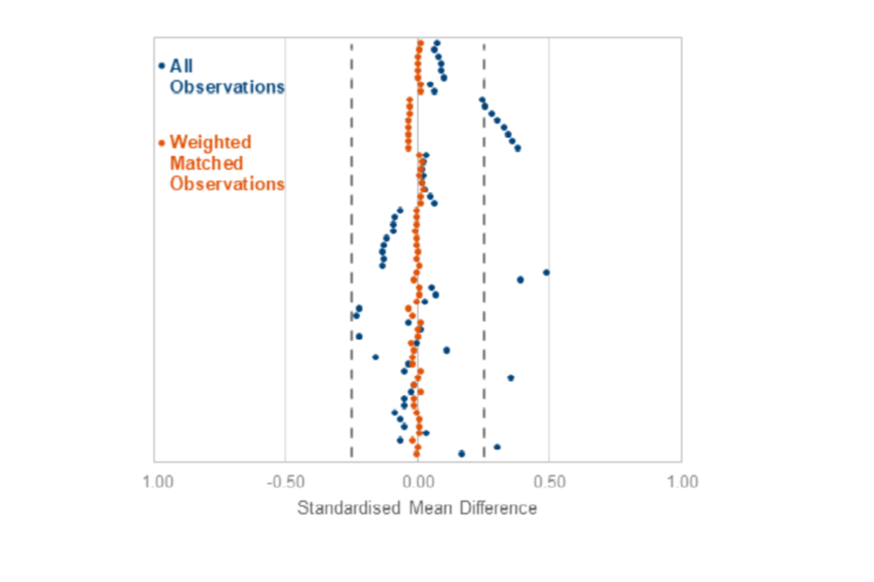
Note: Dotted lines represent an upper and lower limit of +0.25 and -0.25 respectively.

Figure 2.4 further illustrates the effect of matching on minimising the bias on employment history. It shows how, after matching, the UC and legacy groups have very similar employment histories on average. As employment history is a key determinant of employment outcomes following a benefit claim, this further reassures us the matching was successful.

Figure 2.4 Close alignment of employment histories for UC and legacy claimants after matching

Percentage of claimant group in employment each week relative to the week of claim start

We assume we also minimise any unobservable differences between the treatment and comparison groups. This assumption is untestable. We cannot know if, after matching, unobservable differences remain between the treatment and comparison groups which might affect outcomes. However, previous research suggests that controlling for labour market histories implicitly captures a large part of unobservable characteristics such as motivation or other personal traits affecting outcomes (Caliendo and others, 2008).

2.7 Computing the impact

After obtaining our weighted matched sample of treatment and comparison group observations, we can look to analyse the difference in employment outcomes. We take a ‘doubly robust’ approach, fitting a linear regression model on the weighted matched sample where the outcome measure is employment. We use the same covariates used in the propensity score matching procedure and include an indicator for whether the claim was treatment or not. The coefficient on the treatment indicator provides us with the employment impact. As discussed in (Stuart, 2010), matching methods and regression adjustment are complementary. The idea is similar to regression adjustment in randomised experiments where the regression reduces any small residual bias between the treatment and comparison groups. The results of the linear regressions are presented in the following section.

3. Results

In this section we present the results from the linear regressions we run on the weighted matched sample and discuss how we should interpret the results.

3.1 Regression results

Our key outcome is finding employment and we have 2 main measures. Our first measure is the likelihood of employment at some point within a given interval following a claim start, while our second measure is the likelihood of employment at a given interval. We consider these 2 measures at 3 different intervals: 3, 6 and 9 months from the claim start. As set out in section 2.4, we restrict the comparison group sample to legacy benefit claims in Jobcentres where UC rolls out at least 6 months after their legacy benefit claim start date. This effectively means under the 9-month measure, we relax the assumption that the comparison group claimants cannot move to UC in their local area within the tracking period. Table 3.1 defines the outcome measures used.

Table 3.1 Definition of employment outcome measures

Employment outcome	Definition
Within 3 months	Evidence of employment in at least one week of the first 13 following the claim
Within 6 months	Evidence of employment in at least one week of the first 26 following the claim
Within 9 months	Evidence of employment in at least one week of the first 39 following the claim
At 3 months	Evidence of employment in at least one week of weeks 12 to 14 following the claim
At 6 months	Evidence of employment in at least one week of weeks 25 to 27 following the claim
At 9 months	Evidence of employment in at least one week of weeks 38 to 40 following the claim

Table 3.2 below summarises the results based on the above measures. It shows single parents claiming UC are 5.3 percentage points(ppts) more likely to have been in work within 6 months of making a claim compared to claiming legacy benefits. The ‘employed at’ measure shows a similar finding, with Table 3.2 showing single parents claiming UC being 5.5 percentage points more likely to be in work 6 months after making a claim compared to claiming legacy benefits. We find the effect falls between each interval on both measures. Further detail on the regressions can be found in Appendix D.

Table 3.2 Impact within and at different points of a claim: Percentage point(ppt) increase in the likelihood of being in work as a result of claiming UC instead of legacy benefits, Great Britain

Period outcome is observed	Outcome measure percentage points - Employed within	Outcome measure percentage points - Employed at
3 months	6.7 ppts	7.4 ppts
6 months	5.3 ppts	5.5 ppts
9 months	4.5 ppts	4.0 ppts

Note: All estimates are statistically significant at the 1% level. Estimates are rounded to the nearest 0.1 ppt.

We carried out several sensitivity tests to check the robustness of the results, including changing the caliper, adopting different matching methods and testing alternative local labour market controls. We find our headline result holds under different specifications. For further detail, please see Appendix E.

3.2 Regression results by age of the youngest child

This section explores whether the employment impacts of UC on single parents varies by the age of the youngest child. 

As explained in section 2.3, out-of-work single parents with a youngest child aged 3 to 4 have different labour market conditionality expectations under UC compared to the legacy system. Under UC, out-of-work single parents are required to search for work when the youngest child turns 3, while under the legacy system they do not have to search for work until their child turns 5. It is therefore informative to investigate the employment impact separately for single parent claimants whose youngest child is aged 3 to 4 and compare it with those whose youngest child is aged 5 and above. Given the changes in labour market conditionality, we would expect the effects to be higher among the former.

We split our original sample into 2 datasets based on the age of the youngest child in the claim and re-run the PSM procedure. The first dataset contains single parent claimants with a youngest child aged 3 to 4 and the other single parent claimants with a youngest child aged 5 and above. We report on the 6-month headline ‘employed within’ measure in Table 3.3. 

We find UC has a larger employment impact on single parents whose youngest child is aged between 3 and 4. This group is 11.5 percentage points more likely to have been in employment within 6 months of making a claim compared to a group of similar legacy benefit claimants. The effect is smaller for single parents whose youngest child is aged 5 or above. Further detail on the regressions can be found in Appendix D.

Table 3.3 Impact within different points of a claim: Percentage point increase in the likelihood of being in work as a result of claiming UC instead of legacy benefits, by age of the youngest child, Great Britain

Period outcome is observed	Lone parent group ppts - youngest child 3 to 4	Lone parent group ppts - youngest child 5+
3 months	11.8 ppts	4.8 ppts
6 months	11.5 ppts	3.0 ppts
9 months	12.0 ppts	2.1 ppts

Note: All estimates are statistically significant at the 1% level. Estimates are rounded to the nearest 0.1 ppt.

As shown in Table 3.4, despite the sample size being smaller than in the full sample, we still manage to successfully match all treatment observations to comparison observations.

Table 3.4 Size of treatment and comparison group before and after matching and proportion of treatment on support, analysis by age of the youngest child, Great Britain

Single parent group	Matching group	Size before matching	Size after matching	Proportion on support
Youngest child age 3 to 4	Treatment	4,000	4,000	100%
Youngest child age 3 to 4	Comparison	3,700	2,900	N/A
Youngest child age 5 and above	Treatment	13,800	13,800	100%
Youngest child age 5 and above	Comparison	6,600	6,400	N/A

Note: The comparison group sample sizes after matching are before weights are applied. Sample sizes are rounded to the nearest 100. 

We also find the SMDs between the treatment and comparison groups are within the recommended limits, although they are higher on average for claimants with a youngest child aged 3 to 4 than in the main estimates. This is expected given the smaller sample size and the larger difference in characteristics for this group pre-matching. Further details are included in Tables C.2 and C.3 in Appendix C.

3.3 Interpretation

Our results suggest UC has a positive employment effect among single parents relative to the legacy benefit system. This is consistent with the department’s expectations that UC would have an overall positive employment effect due to improved work incentives, a simpler and smoother system, and most importantly for single parents with a youngest child under 5, changes in labour market conditionality. 

The difference in results by age of youngest child suggests conditionality has a much stronger effect on employment outcomes than the other assumed channels. This is consistent with evidence from Lone Parent Obligations: an impact assessment (RR845) - GOV.UK which assessed the effects of single parents losing entitlement to IS. Where applicable, claimants were able to claim JSA or ESA instead, which for many would have resulted in requirements to search for work. The findings suggested 9 months after the estimated loss of IS entitlement, single parents affected by the changes were between 8 and 10 percentage points more likely to be in work.

Since there are no conditionality changes among single parents whose youngest child is 5 or above, we expect the changes in financial work incentives and the simpler and smoother system to be drivers of the results among this group.  

We cannot estimate the extent to which each factor determines outcomes, however the headline result among single parents with children 5 or above is higher than the equivalent estimate among single households without children. This showed single households without children on UC were 2 percentage points more likely to have been in work within 6 months compared to making a claim to JSA. The analysis in this report suggests the same outcome measure for single parents on UC whose youngest child was 5 or above is 3 percentage points.  

We would expect single parents to have a greater response to changes in financial work incentives than single individuals without children, so this difference in impacts is consistent with financial work incentives being a significant driver of the results. In addition, we would expect single parents to be more likely to move between out-of-work and in-work benefits, therefore the higher impact is also consistent with a simpler and smoother system having an employment effect.  

The results appear to decline between intervals which suggests the effect weakens over time for a given cohort. A similar pattern was found when assessing the employment impacts among single households without children. We may expect this as some claimants in the comparison group still find work but take more time to do so than if they were on UC. Employment will still be higher at any given time as new cohorts of claimants continuously join the UC caseload. 

It is important to note the results in our analysis reflect UC policy at the time. Since 2018, there have been several changes to policy which may affect the results if it were possible to repeat the same analysis in a more recent time period. For instance, the government increased existing work allowances in UC by £1,000 per year from April 2019, increased them again by £500 per year and reduced the taper rate by 8 percentage points to 55% from November 2021. If financial work incentives are a particularly important driver, then these changes mean we might expect the employment effects of UC to be higher. 

It is also important to note that our findings are based on a specific group of single parents who made a claim to UC during early 2018. The UC caseload has changed markedly since then. The total UC single parent caseload was 120,000 in January 2018 and tripled to 360,000 by December 2018. Based on the latest available data, the UC single parent caseload was 1.8 million in November 2023.

3.4 Treatment effect on the non-treated

As is typical in propensity score matching analysis, we have estimated the average treatment effect on the treated, where the treatment in this case is a claim to UC. However, this group of single parents in 2018 may not be fully representative of the UC single parent population when UC has fully rolled out.  

We saw from the analysis of characteristics among UC and legacy single parent claimants in section 2.5 how the 2 samples differed. Pre-matching, claimants in the legacy sample were more likely to have claimed out-of-work benefits and were less likely to have been in work prior to their claim start date. To provide further context to our headline outcome measure and to give an indication of how generalisable these results are, we estimate the average treatment effect on the non-treated. 

We reverse the analysis. We use the same specification but set the treatment to be a claim to legacy benefits and match UC single parent claimants to legacy benefit claimants. Following the same approach in the main analysis, we run a linear regression on the weighted matched sample where the outcome is the ‘employed within’ measure. This tells us the employment effect of claiming legacy benefits instead of UC. We find that single parents making a claim to legacy benefits are 7 percentage points less likely to have been in work within 6 months compared to claiming UC. This suggests the employment effect of UC is possibly higher than implied by our headline measure if the legacy benefit sample is more representative of the steady state population. Further detail on this analysis can be found in Appendix F.

References

Austin, P. C. (2011) ‘Optimal caliper widths for propensity‐score matching when estimating differences in means and differences in proportions in observational studies’, Pharmaceutical statistics, 10(2), 150-161. 

Avram, S., Brewer, M. and Salvatori, A. (2013) ‘Lone Parent Obligations: an impact assessment’, Department for Work and Pensions 

Blundell, R., Costa Dias, M., Meghir, C. and Shaw, J. (2016) ‘Female Labor Supply, Human Capital, and Welfare Reform’, Econometrica, Econometric Society, vol. 84, pages 1705-1753, September. 

Caliendo, M., and Kopeinig, S. (2008) ‘Some practical guidance for the implementation of propensity score matching’, Journal of economic surveys, 22(1), 31-72. 

Dehejia, R. H. and Wahba S. (1999) ‘Causal Effects in Non-experimental Studies: Re-evaluating the Evaluation of Training Programs’, Journal of the American Statistical Association, Vol. 94, No. 448, 1053-1062. 

Gelman, A., Hill, J., and Vehtari, A. (2020) ‘Regression and other stories’, Cambridge University Press. 

Lamm, M., Thompson, C. and Yung, Y. (2019) ‘Building a Propensity Score Model with SAS/STAT® Software: Planning and Practice’. 

Rosenbaum, P. R., and Rubin, D. B. (1983) ‘The central role of the propensity score in observational studies for causal effects’, Biometrika, 70(1), 41-55. 

Stuart, E. A. (2010) ‘Matching methods for causal inference: A review and a look forward’, Statistical science: a review journal of the Institute of Mathematical Statistics, 25(1), 1.

Appendices

Appendix A: Data processing

A. 1 UC claim data

UC full service claim data is drawn from the department’s internal UC production data base. This is an extremely rich source of data containing information about a wide range of aspects of UC claims. The data base contains one record per assessment period per UC claim per individual.  

The starting point in building the UC evaluation claim data set is to identify claims on the UC production data base with a valid National Insurance number and claim start date. If either one of these fields are missing it is not possible to merge other key data onto the claim records, such as employment histories and outcomes data from the RTI data. It is also vital that the Jobcentre name is recorded against the claim because we require geographical identifiers so that we can control for area level differences in the analysis.  

It should be noted that only claims that have at least one statement record are retained in the data base and so in practice this means our ‘claims’ are actually equivalent to awards. The term ‘claims’ is used throughout this publication when referring to claims that reach a first award.  

For each claim spell, we use the start date of the first assessment period where the claim was placed in the intensive work search labour market regime, to determine when the claim started for the purpose of this analysis. This start date is then used to filter out claims that lie outside the date range we require for the impact evaluation. Initially we keep one record for each spell. Then, if a person has made multiple claims during the sample period, we only retain one of their claims which we select at random. The final dataset contains one record per claimant. 

Claims made by single parents are identified by making use of a derived variable that classifies family type based on the UC award. This variable is set in each assessment period. We use claims identified as a single parent claim at the claim start.  

As this analysis focus on UC full service claims, claims are excluded if they are identified as direct transfers from a UC live service claim.

A.2 JSA and IS claim data

JSA claim data is drawn from the department’s internal Jobseeker’s Allowance Payment System Atomic Data Store (JSAPS–ADS) data base. IS claims are drawn from the National Benefits Database (NBD). These datasets contain a wide range of information about the claim and the events that take place during the life of the claim. 

As with the UC claim data, the starting point for building the legacy claim evaluation dataset is to identify legacy claims with a valid National Insurance number, claim start date and Jobcentre name. 

There are a number of dates associated with the claim process recorded on the data base, specifically registered date, cleared date, onflow date and claim start date.  We use a field called the ‘claim start date’ to define the start point of legacy claims. This relates to the date entitlement starts from. 

Our UC claim data only includes claims where a statement is generated. This will include some claims with a null payment because the individual claimant is earning enough to not receive an actual payment of UC. JSAPS–ADS includes all claims regardless of whether the claim results in an award. It is possible to identify which claims reach a first award though, so we exclude those claims that do not reach that stage. We also exclude claims with a duration of one day or less which are understood not to be genuine claims.  

UC full service does not replace contributions-based or New Style JSA claims so in order to make a valid comparison group for UC claims, JSA claims must be income-based. Therefore, all contribution-based or new style JSA claims are excluded from the legacy claim data set.  

When it comes to the identification of claims made by single parents, JSAPS–ADS has a marital status field so we can easily identify whether a claim is made by a single person or a couple, but it does not have any fields that enable us to identify the presence of children in the household. Child Benefit data is used to determine whether any children were present at the point of the JSA claim. The combination of marital status and Child Benefit data enables us to identify JSA single parent claims.  For IS claims, a flag to identify IS claims from the National Benefits Database (NBD) is used in combination with the Child Benefit data to identify IS single parent claims.   

As in the UC dataset, if a person has made multiple claims during the sample period, we randomly select one of their claims. The final dataset contains one record per claimant.

A.3 Benefit histories

Benefit claim history is a key determinant of future employment outcomes so for each UC, JSA and IS claim in our data we build a benefit claim history. We use the NBD and the UC Production data base to generate claim histories. We combine data on JSA, IS, ESA and their UC equivalents to provide complete histories for both legacy benefits and UC. The UC production data contains identifiers which provide a proxy mapping to the legacy benefits system based on the circumstances of the claim. This means we can group previous UC spells with their proxy legacy benefit equivalents.  

The period covered by the benefit claim history corresponds to the 2-year period preceding each UC, JSA and IS claim in our data sets. So for a UC claim made on 13 January 2018 we build a benefit claim history covering the period back to 13 January 2016. 

For each of the 105 weeks prior to the UC, JSA or IS claim, a flag is created to indicate whether or not the claimant had a live spell on JSA, IS, ESA or their UC equivalent in that week. For any given week the flag is set if a JSA, IS, ESA or their UC equivalent spell overlaps with at least part of that week. Weekly flags for JSA, IS, ESA and their UC equivalents are aggregated to provide us with a quarterly flag. The quarterly flag is equal to 1 if the claimant has a benefit claim spell in at least one week of that quarter. 

A 2 year flag is also derived to capture whether an individual had any claims to benefits other than JSA, IS, ESA and their UC equivalents at any point in the 2 years prior the claim start.

A.4 Employment histories and outcomes

Past employment history is another key determinant of employment outcomes following a benefit claim. RTI data is used to set flags for each of the 105 weeks before the claim start and the 105 weeks following the claim start to indicate whether the individual was in employment. 

DWP receives a regular feed of RTI payslip data specifically for the employment impact evaluation of UC. The data covers individuals who have claimed UC, JSA or IS at any point from the beginning of 2014. A crucial design feature of this feed is that data continues to be received even after individuals have left the benefits system. This enables us to track the employment outcomes of UC, JSA and IS claimants for as long as is necessary to assess the employment impact of UC. 

We start the processing of the RTI data by filtering out payslips that are missing key fields, for example National Insurance number, payment date and pay frequency. We derive the period of time covered by the payslip and compare the employment spell dates with the start dates of the JSA, IS and UC claims to determine which weeks, relative to the start of the claim, the claimant was in employment.

A.5 Excluding claims with records of employment at the start of their claim 

Since we are interested in the employment effect of UC compared to legacy benefits, we remove claims with full records of employment around their claim start date. Specifically, we exclude treatment and comparison group claims made by single parents who appear to have unbroken employment records in the 4 weeks following their claim start.

A.6 Local average unemployment rate

We use the average unemployment rate in the local authority where the Jobcentre is located to control for differences in local labour market conditions or other local factors affecting the employment outcomes. We source the data from the Office for National Statistics who estimate the rates at a local authority level using data from the Annual Population Survey and the claimant count. The data is available here: Nomis - Official Census and Labour Market Statistics

Appendix B. Variables used in the propensity score matching procedure

Outcome variables	Employment within 13 weeks	Set to 1 if in employment at least 1 week in 3 months following the claim
Outcome variables	Employment within 26 weeks	Set to 1 if in employment at least 1 week in 6 months following the claim
Outcome variables	Employment within 39 weeks	Set to 1 if in employment at least 1 week in 9 months following the claim
Adult personal characteristics	Sex	Set to 1 if female
Adult personal characteristics	Age x	Age of claimant, 1 dummy variable for each of the following age ranges: 16 to 17, 18 to 24, 25 to 29, 30 to 34, 35 to 39, 40 to 44, 45 to 49, 50 to 54, 55 to 59, 60 to 64, 65+
Children information	Age young x	Age of youngest child, one dummy variable for each of the following ages: 3, 4, 5, 6 to 11, 12 to 18
Children information	Child 2	Set to 1 if claimant has 2 children
Benefit information	Month start x	1 dummy variable for each month of claim start (January, February, March, April)
Employment history in the 2 years prior to the claim start	Employment history Q1 to Q8	8 quarterly dummy variables, set to 1 if in employment at least 1 week in that quarter
Benefit history in the 2 years prior to the claim start	IS history Q1 to Q8	8 quarterly dummy variables, set to 1 if claimed IS or UC equivalent at least 1 week in that quarter
Benefit history in the 2 years prior to the claim start	JSA history Q1 to Q8	8 quarterly JSA dummy variables, set to 1 if claimed JSA or UC equivalent at least 1 week in that quarter
Benefit history in the 2 years prior to the claim start	ESA history Q1 to Q8	8 quarterly ESA dummy variables, set to 1 if claimed ESA or UC equivalent at least 1 week in that quarter
Benefit history in the 2 years prior to the claim start	Other benefit	Set to 1 if in receipt of any benefit other than JSA, IS, ESA or UC equivalent in the past 2 years
Benefit history in the 2 years prior to the claim start	Employment programme	Set to 1 if participated in an employment programme in any week in the two years prior to the claim start
Benefit history in the 2 years prior to the claim start	Count of previous benefit spells	Number of benefit spells in JSA, IS, ESA and UC equivalent in the two years prior to the claim start
Benefit history in the 2 years prior to the claim start	Sanction flag	Set to 1 if had any sanctions in the 2 years prior to the claim start
Benefit history in the 2 years prior to the claim start	Claim in previous 4 weeks	Set to 1 if claimed JSA, IS, ESA or UC equivalent in any of the 4 weeks prior to the claim start
Interaction	Age of youngest child 3 X claim in previous 4 weeks	Age of youngest child 3 by whether claimed JSA, IS, ESA or UC equivalent in any of the 4 weeks prior to the claim start
Local labour market control	Average unemployment rate	Average unemployment rate prior to the national rollout of UC full service (2013-15) in the local authority where the Jobcentre is located.

Note: For the analysis by age of the youngest child in the claim, we use larger age bands for the age of adult variables. Specifically, we use under 25, 25 to 49 and 50 plus. Since we are separating the data by the age of youngest child in the claim, we only keep age of youngest child variables relevant to each dataset. We also remove the interaction variable age of youngest child 3 by whether claimed JSA, IS, ESA or UC equivalent in any of the 4 weeks prior to the claim start.

Appendix C. Propensity score matching diagnostics

Table C.1 Propensity score matching diagnostics – full sample

Variable	Mean difference - all obs	Mean difference - weighted matched obs	Standardised Variable Differences (Treated - Comparison) - mean difference - all obs	Standardised Variable Differences (Treated - Comparison) mean difference - weighted matched obs	Standardised Variable Differences (Treated - Comparison) % reduction - weighted matched obs	Variance ratio - all obs	Variance ratio - weighted matched obs
sex	0.015	-0.001	0.048	-0.002	95.610	1.135	0.995
age under 18	0.015	0.000	0.170	0.000	99.810	0.008	1.333
age 18 to 24	0.105	0.002	0.309	0.006	98.150	0.502	0.980
age 25 to 29	-0.024	-0.005	-0.061	-0.012	79.860	1.102	1.018
age 30 to 34	0.015	0.003	0.037	0.009	76.130	1.059	1.013
age 35 to 39	-0.017	0.004	-0.045	0.011	76.050	1.084	0.982
age 40 to 44	-0.021	0.004	-0.062	0.011	81.970	1.142	0.979
age 45 to 49	-0.025	0.000	-0.083	0.002	98.130	1.252	0.996
age 50 to 54	-0.010	-0.002	-0.047	-0.009	80.390	1.216	1.036
age 55 to 59	-0.006	-0.001	-0.043	-0.007	83.090	1.386	1.049
age 60 to 64	-0.002	0.001	-0.022	0.018	20.210	1.350	0.829
age 65 plus	0.000	0.000	-0.009	-0.011	0.000	1.738	2.181
age young 3	0.144	0.002	0.359	0.005	98.510	0.592	0.987
age young 4	-0.013	0.005	-0.048	0.019	60.180	1.158	0.950
age young 5	-0.012	-0.005	-0.033	-0.014	57.930	1.059	1.024
age young 6 to 11	-0.071	-0.007	-0.152	-0.015	90.150	1.129	1.009
age young 12 to 18	0.049	-0.005	0.117	-0.012	90.050	1.172	0.987
child 2	0.000	-0.009	-0.001	-0.018	0.000	1.000	1.008
month start 1	-0.099	0.003	-0.217	0.006	97.220	0.827	1.007
month start 2	0.007	0.002	0.017	0.004	74.400	0.980	0.995
month start 3	-0.012	0.007	-0.028	0.017	41.340	1.035	0.981
month start 4	-0.094	-0.006	-0.229	-0.015	93.400	1.376	1.016
employment history Q1	-0.060	0.000	-0.122	0.001	99.490	1.023	1.000
employment history Q2	-0.064	0.003	-0.128	0.007	94.820	1.024	1.000
employment history Q3	-0.062	0.000	-0.126	0.000	99.660	1.032	1.000
employment history Q4	-0.056	0.001	-0.113	0.002	98.500	1.031	1.000
employment history Q5	-0.044	-0.002	-0.089	-0.004	95.810	1.025	1.001
employment history Q6	-0.042	0.001	-0.085	0.001	98.260	1.025	1.000
employment history Q7	-0.039	0.000	-0.080	0.001	99.320	1.027	1.000
employment history Q8	-0.031	-0.001	-0.063	-0.001	97.830	1.021	1.000
JSA history Q1	0.022	0.005	0.070	0.017	76.250	0.846	0.958
JSA history Q2	0.019	0.006	0.053	0.016	69.250	0.900	0.967
JSA history Q3	0.011	0.009	0.032	0.025	20.650	0.940	0.952
JSA history Q4	0.008	0.007	0.022	0.020	8.080	0.956	0.960
JSA history Q5	0.009	0.004	0.027	0.013	51.870	0.942	0.971
JSA history Q6	0.007	0.006	0.022	0.018	19.350	0.950	0.959
JSA history Q7	0.008	0.006	0.025	0.019	23.540	0.942	0.955
JSA history Q8	0.012	0.004	0.038	0.012	67.520	0.911	0.969
IS history Q1	0.166	-0.013	0.386	-0.030	92.340	0.647	1.061
IS history Q2	0.161	-0.012	0.365	-0.028	92.270	0.693	1.050
IS history Q3	0.155	-0.013	0.350	-0.030	91.430	0.710	1.051
IS history Q4	0.148	-0.014	0.332	-0.031	90.660	0.724	1.052
IS history Q5	0.137	-0.013	0.309	-0.029	90.690	0.739	1.046
IS history Q6	0.127	-0.011	0.284	-0.024	91.620	0.760	1.036
IS history Q7	0.116	-0.011	0.261	-0.024	90.880	0.774	1.036
IS history Q8	0.112	-0.010	0.251	-0.022	91.050	0.778	1.034
ESA history Q1	0.025	0.006	0.068	0.015	78.240	0.888	0.973
ESA history Q2	0.020	0.006	0.054	0.015	72.500	0.907	0.972
ESA history Q3	0.033	0.002	0.103	0.005	95.240	0.780	0.986
ESA history Q4	0.029	0.001	0.094	0.005	95.110	0.785	0.986
ESA history Q5	0.028	0.002	0.092	0.008	91.360	0.781	0.976
ESA history Q6	0.024	0.002	0.082	0.008	90.090	0.801	0.975
ESA history Q7	0.020	0.003	0.068	0.010	85.330	0.825	0.969
ESA history Q8	0.022	0.005	0.077	0.016	79.280	0.801	0.950
other benefit	0.014	0.002	0.057	0.009	83.780	0.812	0.963
employment programme	0.019	0.003	0.075	0.012	84.290	0.779	0.957
count previous benefit spells	-0.247	-0.037	-0.215	-0.032	84.960	0.987	0.898
sanction flag	0.005	0.000	0.032	0.001	97.200	0.806	0.993
claim previous 4 weeks	0.192	-0.005	0.393	-0.010	97.420	0.932	1.006
age young 3 X claim previous 4 weeks	0.168	0.001	0.493	0.001	99.700	0.322	0.992
average unemployment rate	-0.273	0.025	-0.130	0.012	90.830	0.813	0.822

Table C.2 Propensity score matching diagnostics – age of youngest child 3 to 4

Variable	Mean difference - all obs	Mean difference - weighted matched obs	Standardised Variable Differences (Treated - Comparison) - mean difference - all obs	Standardised Variable Differences (Treated - Comparison) mean difference - weighted matched obs	Standardised Variable Differences (Treated - Comparison) % reduction - weighted matched obs	Variance ratio - all obs	Variance ratio - weighted matched obs
sex	0.014	-0.005	0.060	-0.019	67.990	1.246	0.942
age under 25	0.114	-0.005	0.254	-0.012	95.400	0.781	1.017
age 25 to 49	-0.112	0.005	-0.249	0.012	95.250	0.794	1.016
age 50 plus	-0.001	0.000	-0.015	-0.001	92.410	1.185	1.012
age young 3	0.177	-0.037	0.395	-0.082	79.330	1.442	0.971
age young 4	0.177	-0.037	0.395	-0.082	79.330	1.442	0.971
child 2	-0.017	0.005	-0.033	0.011	67.700	1.008	0.998
month start 1	-0.088	-0.036	-0.195	-0.081	58.560	0.832	0.914
month start 2	0.020	0.007	0.046	0.016	65.730	0.948	0.981
month start 3	-0.012	-0.004	-0.028	-0.009	66.830	1.034	1.011
month start 4	-0.096	-0.039	-0.232	-0.095	58.990	1.373	1.112
employment history Q1	-0.163	0.017	-0.337	0.035	89.490	1.151	0.999
employment history Q2	-0.146	0.003	-0.302	0.006	97.980	1.142	0.999
employment history Q3	-0.139	-0.003	-0.290	-0.006	97.960	1.164	1.001
employment history Q4	-0.134	-0.006	-0.281	-0.012	95.640	1.178	1.004
employment history Q5	-0.114	-0.005	-0.239	-0.011	95.480	1.155	1.004
employment history Q6	-0.106	-0.004	-0.222	-0.009	96.130	1.144	1.003
employment history Q7	-0.094	-0.010	-0.199	-0.021	89.350	1.138	1.009
employment history Q8	-0.073	-0.013	-0.153	-0.028	81.800	1.097	1.013
JSA history Q1	-0.008	0.004	-0.049	0.023	52.840	1.350	0.892
JSA history Q2	-0.007	0.003	-0.047	0.017	64.590	1.334	0.920
JSA history Q3	-0.007	0.000	-0.050	0.001	98.590	1.382	0.996
JSA history Q4	-0.010	0.004	-0.068	0.026	62.090	1.578	0.880
JSA history Q5	-0.003	0.009	-0.024	0.062	0.000	1.167	0.731
JSA history Q6	-0.002	0.007	-0.012	0.051	0.000	1.084	0.754
JSA history Q7	-0.006	0.005	-0.043	0.032	24.920	1.336	0.843
JSA history Q8	-0.001	0.004	-0.005	0.024	0.000	1.035	0.870
IS history Q1	0.335	-0.004	0.711	-0.008	98.930	1.060	1.005
IS history Q2	0.310	-0.009	0.655	-0.019	97.050	1.097	1.010
IS history Q3	0.292	-0.005	0.613	-0.010	98.370	1.077	1.005
IS history Q4	0.275	-0.007	0.573	-0.014	97.520	1.045	1.007
IS history Q5	0.254	-0.014	0.526	-0.029	94.460	1.000	1.017
IS history Q6	0.230	-0.016	0.472	-0.032	93.130	0.987	1.018
IS history Q7	0.207	-0.016	0.423	-0.033	92.290	0.959	1.019
IS history Q8	0.197	-0.008	0.403	-0.016	95.950	0.940	1.010
ESA history Q1	-0.031	0.007	-0.141	0.031	78.220	1.820	0.914
ESA history Q2	-0.029	0.011	-0.134	0.048	64.320	1.748	0.872
ESA history Q3	-0.005	0.011	-0.026	0.059	0.000	1.133	0.794
ESA history Q4	-0.003	0.008	-0.015	0.044	0.000	1.077	0.830
ESA history Q5	0.006	0.008	0.034	0.040	0.000	0.846	0.821
ESA history Q6	0.007	0.004	0.039	0.022	45.210	0.825	0.895
ESA history Q7	0.008	0.004	0.041	0.023	43.580	0.819	0.889
ESA history Q8	0.009	0.004	0.046	0.020	57.250	0.801	0.903
other benefit	0.034	0.008	0.148	0.036	75.440	0.558	0.833
employment programme	0.017	0.003	0.104	0.018	82.780	0.528	0.865
count previous benefit spells	-0.086	-0.034	-0.104	-0.041	60.840	1.755	0.872
sanction flag	0.001	0.001	0.015	0.011	25.520	0.749	0.800
claim previous 4 weeks	0.334	0.001	0.711	0.002	99.780	1.114	0.999
average unemployment rate	-0.177	-0.046	-0.085	-0.022	74.240	0.829	0.837

Table C.3 Propensity score matching diagnostics – age of youngest child 5 and over

Variable	Mean difference - all obs	Mean difference - weighted matched obs	Standardised Variable Differences (Treated - Comparison) - mean difference - all obs	Standardised Variable Differences (Treated - Comparison) mean difference - weighted matched obs	Standardised Variable Differences (Treated - Comparison) % reduction - weighted matched obs	Variance ratio - all obs	Variance ratio - weighted matched obs
sex	0.004	-0.001	0.012	-0.002	79.910	1.027	0.995
age under 25	0.084	-0.001	0.307	-0.003	99.070	0.363	1.018
age 25 to 49	-0.077	-0.002	-0.199	-0.006	96.890	0.719	0.987
age 50 plus	-0.007	0.003	-0.025	0.011	57.470	1.069	0.974
age young 5	0.028	-0.001	0.065	-0.003	94.950	0.925	1.004
age young 6 to 11	-0.017	-0.003	-0.034	-0.006	82.100	1.007	1.001
age young 12 to 18	0.011	-0.004	0.023	-0.010	58.940	1.019	0.993
child 2	-0.004	-0.009	-0.008	-0.019	0.000	1.004	1.009
month start 1	-0.107	0.003	-0.233	0.006	97.260	0.822	1.008
month start 2	0.000	-0.001	0.000	-0.003	0.000	1.000	1.003
month start 3	-0.013	0.006	-0.030	0.014	51.690	1.037	0.984
month start 4	-0.094	-0.002	-0.230	-0.005	97.840	1.382	1.005
employment history Q1	-0.003	0.004	-0.005	0.008	0.000	1.000	1.000
employment history Q2	-0.013	0.004	-0.025	0.008	68.350	1.002	1.000
employment history Q3	-0.013	-0.003	-0.026	-0.005	80.230	1.003	1.001
employment history Q4	-0.004	-0.002	-0.008	-0.004	50.010	1.001	1.001
employment history Q5	0.005	-0.003	0.011	-0.007	36.710	0.999	1.001
employment history Q6	0.005	-0.002	0.009	-0.004	59.430	0.999	1.001
employment history Q7	0.003	-0.001	0.006	-0.002	70.650	0.999	1.000
employment history Q8	0.003	-0.002	0.007	-0.004	36.890	0.999	1.001
JSA history Q1	0.059	0.004	0.163	0.010	93.570	0.732	0.975
JSA history Q2	0.063	0.008	0.157	0.021	86.930	0.792	0.964
JSA history Q3	0.053	0.006	0.132	0.015	88.440	0.825	0.974
JSA history Q4	0.046	0.007	0.118	0.017	85.910	0.831	0.970
JSA history Q5	0.043	0.006	0.113	0.014	87.210	0.824	0.972
JSA history Q6	0.038	0.006	0.102	0.017	83.280	0.831	0.966
JSA history Q7	0.039	0.008	0.108	0.023	78.690	0.815	0.952
JSA history Q8	0.041	0.008	0.115	0.023	79.910	0.799	0.950
IS history Q1	0.026	-0.003	0.074	-0.009	88.160	0.856	1.021
IS history Q2	0.030	-0.002	0.082	-0.005	93.910	0.860	1.011
IS history Q3	0.032	-0.002	0.086	-0.006	93.550	0.861	1.011
IS history Q4	0.031	-0.001	0.082	-0.003	96.120	0.870	1.006
IS history Q5	0.030	-0.001	0.077	-0.004	95.100	0.880	1.007
IS history Q6	0.028	0.002	0.072	0.004	94.080	0.893	0.993
IS history Q7	0.026	0.002	0.067	0.004	94.210	0.902	0.994
IS history Q8	0.027	0.001	0.068	0.003	95.120	0.901	0.995
ESA history Q1	0.081	0.001	0.195	0.001	99.260	0.772	0.998
ESA history Q2	0.071	0.004	0.174	0.011	93.910	0.786	0.982
ESA history Q3	0.069	0.004	0.194	0.012	93.670	0.680	0.968
ESA history Q4	0.060	0.002	0.176	0.007	96.270	0.685	0.982
ESA history Q5	0.054	0.003	0.161	0.010	93.690	0.697	0.972
ESA history Q6	0.047	0.004	0.144	0.012	91.890	0.718	0.968
ESA history Q7	0.040	0.004	0.124	0.012	90.080	0.743	0.965
ESA history Q8	0.042	0.004	0.132	0.011	91.380	0.723	0.967
other benefit	0.007	0.002	0.028	0.010	64.320	0.905	0.964
employment programme	0.033	0.002	0.113	0.007	93.770	0.723	0.976
count previous benefit spells	-0.360	-0.033	-0.286	-0.026	90.820	0.827	1.046
sanction flag	0.011	0.001	0.065	0.009	86.450	0.687	0.941
claim previous 4 weeks	0.111	0.000	0.226	-0.001	99.700	0.923	1.000
average unemployment rate	-0.348	0.060	-0.165	0.028	82.780	0.806	0.838

Appendix D. Regression results

The tables below present the regression outputs for the coefficient on the treatment indicator for the different measures and samples.

Table D.1 Regression coefficients for the treatment indicator at different intervals, ‘employed within’ measure – full sample 

	Estimate	Standard error	t Value	Pr > |t|	95% confidence interval	95% confidence interval
Within 3 months	0.067	0.006	10.340	<.0001	0.054	0.079
Within 6 months	0.053	0.007	7.950	<.0001	0.040	0.065
Within 9 months	0.045	0.007	6.790	<.0001	0.032	0.058

Note: Estimates are significant at the 1% level. We use the proc surveyreg procedure in SAS to carry out the regression on the matched weighted sample. Standard errors are robust and obtained by clustering by individual observations. For further detail see: The SURVEYREG Procedure (sas.com) 

Table D.2 Regression coefficients for the treatment indicator at different intervals, ‘employed at’ measure – full sample

	Estimate	Standard error	t Value	Pr > |t|	95% confidence interval	95% confidence interval
At 3 months	0.074	0.006	11.550	<.0001	0.062	0.087
At 6 months	0.055	0.007	8.170	<.0001	0.042	0.068
At 9 months	0.040	0.007	5.870	<.0001	0.027	0.054

Note: Estimates are significant at the 1% level. We use the proc surveyreg procedure in SAS to carry out the regression on the matched weighted sample. Standard errors are robust and obtained by clustering by individual observations. For further detail see: The SURVEYREG Procedure (sas.com) 

Table D.3 Regression coefficients for the treatment indicator at different intervals, ‘employed within’ measure – single parents with a youngest child aged 3 to 4 sample

Treated age 3 to 4	Estimate	Standard error	t Value	Pr > |t|	95% confidence interval	95% confidence interval
Within 3 months	0.118	0.012	9.730	<.0001	0.094	0.142
Within 6 months	0.115	0.013	8.990	<.0001	0.090	0.139
Within 9 months	0.120	0.013	9.270	<.0001	0.095	0.145

Note: Estimates are significant at the 1% level. We use the proc surveyreg procedure in SAS to carry out the regression on the matched weighted sample. Standard errors are robust and obtained by clustering by individual observations. For further detail see: The SURVEYREG Procedure (sas.com)

Table D.4 Regression coefficients for the treatment indicator at different intervals, ‘employed within’ measure – single parents with a youngest child 5 and above sample

Treated age 5 +	Estimate	Standard error	t Value	Pr > |t|	95% confidence interval	95% confidence interval
Within 3 months	0.048	0.008	6.180	<.0001	0.032	0.063
Within 6 months	0.030	0.008	3.850	0.000	0.015	0.046
Within 9 months	0.021	0.008	2.660	0.008	0.005	0.036

Note: Estimates are significant at the 1% level. We use the proc surveyreg procedure in SAS to carry out the regression on the matched weighted sample. Standard errors are robust and obtained by clustering by individual observations. For further detail see: The SURVEYREG Procedure (sas.com)

Appendix E. Sensitivity checks

This section presents the sensitivity and robustness checks we conducted. Firstly, we assessed the extent to which our employment impact estimates varied with changes to our model specification. Secondly, we checked whether there were any systematic differences between the areas we selected for the analysis. Finally, we analysed whether the estimates were sensitive to how we accounted for local area differences. The details of these checks are set out in the 3 sub-sections below.

E 1. Testing different model specifications

The table below sets out the different model specifications we tested, including an explanation of the change and the results. We use the same model as used in the main analysis and vary the specification as described in each test. The outcome measure is the ‘employed within’ measure at the 6 month interval. 

Table E.1 Summary of different model specifications tested

Adjustment in specification	Explanation	Findings
1. Adjusting the k in propensity score matching (PSM)	The k specifies the number of matching comparison group units for each treated unit. We use proc psmatch in SAS which performs k separate loops of matching for treated units. In each loop, the nearest comparison group unit is sequentially matched to each treated unit. We tested k=1,3,4,5,6 and 8.	The impact estimate varied between 5.2ppts and 5.5ppts.
2. Adjusting the caliper	For all matching methods, you can specify a caliper width, which imposes a restriction on the quality of the matches. The difference in propensity score between the treated unit and its matching comparison group unit must be less than or equal to the caliper width. We tested calipers of 0.0005, 0.05, 0.1, 0.2 and 0.5.	The impact estimate varied between 5.2ppts and 5.3ppts.
3. Testing different matching methods	We tested: Adaptive procedure – it models the propensity scores by automatically selecting the appropriate nonlinear trends and interaction effects (Lamm and others, 2019). It creates an overfitted model first, then refines it with a backward selection technique. Greedy – the greedy matching method selects the comparison group unit whose propensity score best matches the propensity score of each treated unit. Greedy nearest neighbour matching is done sequentially and without replacement. Adding the seed sub option orders the treated units in random order of the propensity score.	The adaptive procedure provided an impact estimate of 4.7ppts and the greedy matching approach provided an impact estimate of 5.7ppts.
4. Exact matching	We tested the impact of applying exact matching on key variables such as local unemployment rate and age of the youngest child. This option involves matching treatment and comparison observations that have the same exact value on a specific set of covariates. These options led to a deterioration of the matching quality.	Exact matching on the age of the youngest child 3 and 4 provided an impact estimate of 5.0ppts and exact matching on local unemployment rate provided an impact estimate of 4.7ppts.
6. Retaining comparison group observations in areas that move to UC before the headline outcome is observed	We tested the impact of only excluding comparison group claims in areas that rolled out to UC one month after the claim start (as opposed to 6 months as in the main model). This doubled the size of the comparison group sample from 10,300 to 20,400 but meant that just under 3% of them moved to UC within the 6-month tracking period.	Modifying the restrictions on the comparison group provided an impact estimate of 5.6ppts.
7. Testing the sample period date range	We varied the sample period date range to assess whether the period that we had chosen influenced the outcome of the analysis.	Using a March to May 2018 sampling period provided an impact estimate of 5.1ppts.

Note: The outcome measure is the ‘employed within’ measure at the 6-month interval. We use the proc psmatch procedure in SAS to carry out the propensity score matching. For further detail see: The PSMATCH Procedure (sas.com).  

Overall, we find that the UC employment impacts for single parents do not vary by much when we make different data and modelling choices, and so we conclude that our analysis is robust to these observables.

E 2. Testing geographical differences

It is possible that the higher outcomes observed among UC claims might be partly driven by unobserved geographical differences, such as differences in Jobcentre performance or other local factors not sufficiently captured by the local unemployment rate variable included in the model.  

This would indicate that the matched comparison group would not be a robust estimate of what the outcomes of matched UC claimants would have been had they not received UC. This bias cannot be formally tested because it is impossible to know what the outcomes of UC claimants would have been had UC not rolled out.  

However, it is possible to produce evidence to support this assumption using data from before UC full service began national rollout. To do this, we re-estimate the PSM model for claims made between April 2014 and October 2014. Specifically, we compare legacy benefit claims made in the Jobcentres from the treatment group from the main analysis with those made in Jobcentres from the matched comparison group.  

The intuition behind this ‘placebo test’ is that any difference between outcomes among legacy benefit claims in the 2 groups would indicate UC is not the only factor driving the employment impact. We replicate the main analysis, using the PSM to ensure balance between the 2 groups of legacy benefit claims, and fit a linear regression to estimate the employment impact using the ‘employed within 6 months’ outcome measure.  

The analysis found that the difference in employment outcomes between claimants in treatment and comparison group Jobcentres was close to zero (-0.6 percentage points)^{[footnote 5]}. In other words, prior to the treatment group Jobcentres in our main analysis rolling out to UC, single parents making claims to legacy benefits in those areas had marginally poorer employment outcomes compared to those in comparison group areas. This suggests the results from our main analysis are not driven by unobservable geographical differences.

E 3. Testing alternative local level controls

We checked the sensitivity of the results to the choice of variable selected to control for local level effects. We re-ran the model by replacing the local unemployment rate with a set of dummy variables representing one of 14 local labour market types for the local authority each individual resides in. These local labour market types, referred to as clusters, are based on grouping local authorities together depending on how similar they are according to the following underlying labour market characteristics (based on variables a to f outlined below). 

a.  Claimant Count (NOMIS Claimant Count) 

b.  Employment rate (NOMIS APS) 

c.  Equality Act /work-limiting disability rate (NOMIS APS) 

d.  NVQ4+ rate (NOMIS APS) 

e.  Musculo- skeletal Condition rate  (Office for Health Improvement & Disparities public health profiles) 

f.  Rate of mental health issues  (Office for Health Improvement & Disparities public health profiles) 

We used geographic data in the Customer Information System, taking addresses of claimants recorded at the time of their claim start to identify the local authority of residence. If this was not available, we took the first recorded address after claim start. We excluded addresses with no local authority entry (mostly international addresses). Where multiple addresses were recorded, we identified a primary address.  

Once the local authority of residence had been determined we were able to match in the local labour market type for each individual in the dataset. 

We re-ran the PSM model using the ‘employed within’ measure and the 6-month tracking period. We found that the UC employment impacts among single parents was 5.5 percentage points. We therefore conclude our analysis is robust to changes in how we control for local level differences.

Appendix F. 1. Treatment effect on the non-treated

As an additional sensitivity check we reversed the analysis and assessed the effects of UC on the comparison group, which is referred to as the average treatment effect on the non-treated. This tells us what the employment effect is from making a claim to legacy benefits instead of UC. 

The rationale for this was to better understand the extent to which our headline results are generalisable for the single parent population. The UC caseload at the time of the analysis is not necessarily reflective of the steady state population, as the UC caseload was gradually increasing. The total UC single parent caseload was 120,000 in January 2018 and tripled to 360,000 by December 2018. Based on the latest available data, the UC single parent caseload was 1.8 million in November 2023.  

We use the same PSM specification from our main analysis but we switch the treatment to a claim to legacy benefits. We therefore match UC claims to legacy benefit claims, reversing the approach taken in our main analysis. We achieve a high-quality match with 99% of treatment observations on support and SMDs all within the relevant thresholds. We then run a linear regression to estimate the employment effect. 

The results suggest single parents claiming legacy benefits are 7 percentage points less likely to have been in work within 6 months of making a claim than if they had claimed UC. This suggests the employment effect of UC is possibly higher than implied by our headline measure if the legacy benefit population is more representative of the steady state population. See regression results for the treatment indicator, sample sizes and propensity score matching diagnostics in Tables F.1, F.2 and F.3 below.

Table F.1 Regression coefficient to estimate the percentage point increase in the likelihood of being in work as a result of claiming legacy benefits instead of UC – single parents

Treated: claim to legacy benefits	Estimate	Standard error	t value	Pr > |t|	95% confidence interval	95% confidence interval
In employment within 6 months	-0.070	0.007	-10.640	<.0001	-0.083	-0.057

Note: Estimates are significant at the 1% level. We use the proc surveyreg procedure in SAS to carry out the regression on the matched weighted sample. Standard errors are robust and obtained by clustering by individual observations. For further detail see: The SURVEYREG Procedure (sas.com)

Table F.2 Size of treatment (legacy benefits) and comparison group (UC) before and after matching and proportion of treatment on support

Matching group	Size before matching	Size after matching	Proportion on support
Treatment	10,300	10,200	99%
Comparison	17,800	13,400	N/A

Note: The comparison group sample size after matching is before weights are applied.   Sample sizes are rounded to the nearest 100. 

Table F.3 Propensity score matching diagnostics – treatment effect on the non-treated

	Mean difference - All obs	Mean difference - weighted matched obs	Standardised Variable Differences (Treated – Comparison Group) - mean difference - all obs	Standardised Variable Differences (Treated – Comparison Group) - mean difference - weighted matched obs	Standardised Variable Differences (Treated – Comparison Group) - % reduction - weighted matched obs	Variance ratio - all obs	Variance ratio - weighted matched obs
sex	-0.015	0.002	-0.048	0.006	87.570	0.881	1.017
age under 18	-0.015	0.000	-0.170	0.001	99.320	128.440	0.875
age 18 to 24	-0.105	0.004	-0.309	0.011	96.290	1.994	0.985
age 25 to 29	0.024	-0.005	0.061	-0.014	77.580	0.908	1.024
age 30 to 34	-0.015	0.000	-0.037	0.001	96.970	0.944	1.002
age 35 to 39	0.017	0.002	0.045	0.006	87.040	0.922	0.989
age 40 to 44	0.021	0.000	0.062	0.000	99.300	0.876	0.999
age 45 to 49	0.025	0.001	0.083	0.003	96.440	0.799	0.991
age 50 to 54	0.010	-0.001	0.047	-0.006	87.920	0.822	1.027
age 55 to 59	0.006	-0.001	0.043	-0.006	86.500	0.722	1.054
age 60 to 64	0.002	0.001	0.022	0.010	56.450	0.741	0.869
age 65 plus	0.000	0.000	0.009	-0.003	65.640	0.576	1.333
age young 3	-0.144	-0.002	-0.359	-0.004	98.910	1.691	1.004
age young 4	0.013	0.002	0.048	0.006	86.890	0.864	0.980
age young 5	0.012	-0.002	0.033	-0.006	82.480	0.944	1.011
age young 6 to 11	0.071	0.000	0.152	0.001	99.580	0.886	0.999
child 2	0.000	-0.009	0.001	-0.018	0.000	1.000	1.008
month start 1	0.099	-0.001	0.217	-0.003	98.770	1.209	0.998
month start 2	-0.007	-0.001	-0.017	-0.002	89.280	1.021	1.002
month start 3	0.012	-0.005	0.028	-0.011	60.700	0.966	1.014
month start 4	0.094	0.004	0.229	0.011	95.400	0.727	0.980
JSA history Q1	-0.022	0.010	-0.070	0.033	52.830	1.182	0.936
JSA history Q2	-0.019	0.010	-0.053	0.027	48.800	1.111	0.954
JSA history Q3	-0.011	0.010	-0.032	0.027	15.560	1.064	0.954
JSA history Q4	-0.008	0.006	-0.022	0.018	15.900	1.046	0.966
JSA history Q5	-0.009	0.005	-0.027	0.014	46.960	1.062	0.971
JSA history Q6	-0.007	0.008	-0.022	0.024	0.000	1.053	0.950
JSA history Q7	-0.008	0.010	-0.025	0.031	0.000	1.062	0.936
JSA history Q8	-0.012	0.009	-0.038	0.027	27.970	1.097	0.942
IS history Q1	-0.166	-0.017	-0.386	-0.040	89.560	1.545	1.027
IS history Q2	-0.161	-0.017	-0.365	-0.038	89.550	1.444	1.023
IS history Q3	-0.155	-0.020	-0.350	-0.045	87.190	1.408	1.028
IS history Q4	-0.148	-0.017	-0.332	-0.039	88.230	1.382	1.024
IS history Q5	-0.137	-0.016	-0.309	-0.036	88.300	1.354	1.024
IS history Q6	-0.127	-0.015	-0.284	-0.034	87.870	1.316	1.023
IS history Q7	-0.116	-0.014	-0.261	-0.032	87.850	1.292	1.023
IS history Q8	-0.112	-0.013	-0.251	-0.028	88.710	1.285	1.021
age young 12 to 18	-0.049	-0.002	-0.117	-0.004	96.410	0.853	0.994
ESA history Q1	-0.025	0.015	-0.068	0.041	39.490	1.126	0.941
ESA history Q2	-0.020	0.016	-0.054	0.043	20.360	1.102	0.936
ESA history Q3	-0.033	0.013	-0.103	0.042	59.380	1.282	0.923
ESA history Q4	-0.029	0.013	-0.094	0.042	54.750	1.274	0.917
ESA history Q5	-0.028	0.011	-0.092	0.038	59.150	1.281	0.922
ESA history Q6	-0.024	0.009	-0.082	0.030	63.790	1.249	0.936
ESA history Q7	-0.020	0.008	-0.068	0.027	60.180	1.212	0.938
ESA history Q8	-0.022	0.007	-0.077	0.026	66.940	1.249	0.941
count previous benefit spells	0.247	-0.070	0.215	-0.061	71.620	1.013	1.020
average unemployment rate	0.273	0.030	0.130	0.015	88.880	1.230	1.206
employment history Q1	0.060	0.003	0.122	0.007	94.430	0.978	0.998
employment history Q2	0.064	0.002	0.128	0.004	96.620	0.977	0.999
employment history Q3	0.062	-0.002	0.126	-0.004	97.190	0.969	1.001
employment history Q4	0.056	-0.004	0.113	-0.007	93.540	0.970	1.003
employment history Q5	0.044	-0.004	0.089	-0.007	91.840	0.976	1.003
employment history Q6	0.042	-0.007	0.085	-0.014	83.320	0.976	1.005
employment history Q7	0.039	-0.005	0.080	-0.010	87.010	0.974	1.004
employment history Q8	0.031	-0.007	0.063	-0.015	76.470	0.979	1.006
sanction flag	-0.005	0.001	-0.032	0.009	72.240	1.240	0.950
employment prog f	-0.019	0.004	-0.075	0.016	79.160	1.283	0.958
other benefits	-0.014	0.000	-0.057	-0.002	97.000	1.232	1.006
claim previous 4 weeks	-0.192	-0.002	-0.393	-0.005	98.840	1.073	0.999
age young 3 X claim previous 4 weeks	-0.168	-0.003	-0.493	-0.009	98.160	3.109	1.010

Note: We use the proc psmatch procedure in SAS to carry out the propensity score matching. For further detail see: The PSMATCH Procedure (sas.com)

1. See (Blundell and others, 2016) ↩

2. For simplicity UC refers to the UC full service for the rest of the report unless stated otherwise ↩

3. We do not restrict claimants moving between UC and legacy areas. We find only 0.4% of legacy cases make a claim to UC and less than 0.1% of UC cases make a claim to legacy benefits within the 6-month tracking period. ↩

4. As recommended in (Austin, 2011), we use a caliper of 0.20. ↩

5. This result was significant at the 1% level. ↩