DLUHC appraisal guide

Question 1

Foreword

Accepted Answer

In 2016 the Department for Communities and Local Government (DCLG) published the first edition of its Appraisal Guide. The aim was to ensure that Ministers and other decision makers have robust evidence on value for money when making policy and investment decisions.

That Guide has been widely used within the Department, which is now the Department for Levelling Up, Housing and Communities (DLUHC), other government departments and at local level, to inform spending decisions on housing, commercial property and land use and funding decisions by local authorities.

However, two changes have occurred recently which mean it is necessary to update and develop the Appraisal Guide so that it continues to provide relevant, robust and trusted advice:

In November 2020 HMT published a revised Green Book. This emphasised the importance of considering all objectives and impacts (including non-monetised impacts) and making fuller use of place based analysis in VfM assessments;
The Levelling Up White Paper published in February 2022 places much greater focus on reducing geographical disparities, identifying six key capitals as fundamental to determining area performance, and twelve key missions which will support development of those capitals in left behind areas to deliver levelling up.

This updated Appraisal Guide responds to both these developments, providing additional advice on how to rigorously assess VfM and a greater focus on spatial and distributional impacts including wider regeneration of areas.

I am therefore very pleased to recommend the use of this Guide as a means of helping to deliver better evidenced-based policy making. The Guide is a living document and I look forward to future improvements that should make it even more helpful.

I would like to thank every analyst and economist in the Department (including those from Homes England) who have contributed to it, with a particular thanks to Andrew Charlesworth-May who has led the delivery of this important update. I would also like to thank Michael Spackman, Professor Peter Tyler and Professor Henry Overman who have provided invaluable comments to support its improvement.

Stephen Aldridge
Director for Analysis and Data
Department for Levelling Up Housing and Communities

Question 2

List of abbreviations

Accepted Answer

AH: Affordable Housing

AONB: Area of Outstanding Natural Beauty

AST: Appraisal Summary Table

BAU: Business as Usual

BCR: Benefit Cost Ratio

BRE: Building Research Establishment

CORE: Continuous Recording of Lettings and Sales in England (DLUHC survey)

GCMA: Greater Manchester Combined Authority

GHG: Greenhouse Gas

GVA: Gross Value Added

HE: Homes England

LVU: Land Value Uplift

MV: Market value

NAO: National Audit Office

NPSV: Net present social value

OB: Optimism bias

PDL: Previously Developed Land

PRP: Private Registered Providers

PRS: Private Rented Sector

PVB: Present Value of Benefits

PVC: Present Value of Costs

PWF: Preferred Way Forward

SR: Spending Review

SRS: Social Rented Sector

TA: Temporary Accommodation

VfM: Value for Money

VOA: Valuation Office Agency

Question 3

DLUHC appraisal group

Accepted Answer

The DLUHC appraisal group is responsible for overseeing the development of appraisal guidance in DLUHC and ensuring it is communicated and applied effectively within DLUHC and across partner organisations. The group covers all areas of appraisal relevant to DLUHC and Homes England.

Stephen Aldridge, Chief Analyst at DLUHC
Stephen Meredith, Deputy Director, Housing and Planning Analysis and Chair of Appraisal Group
Andrew Charlesworth-May, Lead Co-ordinator and Analyst for Appraisal Guide
Andrew Wallis, Chief Economist, Homes England
Jo Brotherhood, Head of Economics, Homes England
Ben Toogood, Deputy Director, Local Policy Analysis
Zebedee Nartey, Deputy Director, Local Growth Analysis
Catherine Barham, Deputy Director, Vulnerable People, Data and Evaluation
Paul Vickers, Deputy Director, Safer and Greener Buildings Analysis
Emily McGovern, Head of Homelessness and Rough Sleeping Data and Statistics
Amy Sippitt, Head of Elections Research and Analysis
Frank Brocek, Senior Economist, Union Devolution Research and Analysis
Thomas Annable, Senior Economist, Safer and Greener Buildings Analysis
David Craine, Senior Economist, Safer and Greener Buildings Analysis
Chloe Maycock, Senior Economist, Local Growth Analysis
Stephen Smith, Senior Economist, Local Policy Analysis
Gemma Weston, Senior Economist, Housing and Planning Analysis
Robert Mills, Senior Economist, Housing and Planning Analysis
Lan-Ho Man, Principal Research Officer, Vulnerable People, Data and Evaluation

Question 4

1.  Introduction

Accepted Answer

The role of economic appraisal

1.1 Appraisal is an essential part of the policy making process, represented by HM Treasury’s Green Book ROAMEF framework in the figure below. It is about finding the best way to meet policy objectives.

Figure 1: ROAMEF model

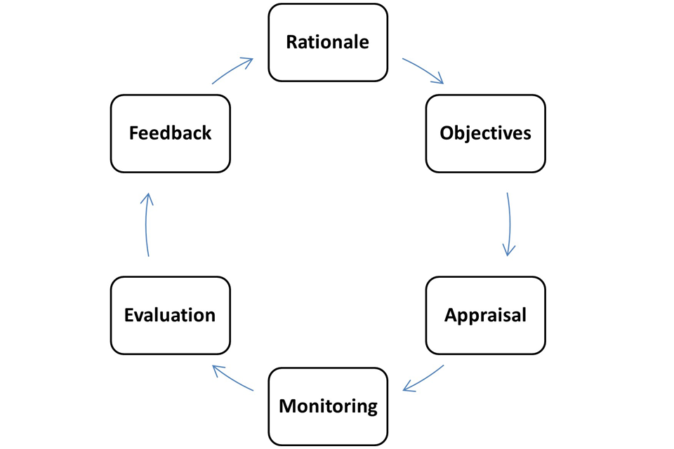
The six components are Rationale, Objectives, Appraisal, Monitoring, Evaluation and Feedback.

1.2 Appraisal is a two step process, conducted through longlisting then shortlisting analysis, following HM Treasury’s Five Case Business Case model^{[footnote 1]}.

1.3 DLUHC uses the Green Book for its appraisal. This guide sets out specific appraisal issues that arise in DLUHC policy areas and is focused on the economic dimension of the business case, providing specific guidance on the quantification of impacts in the economic dimension. The appraisal approaches set out are also applicable to the assessment of options in Impact Assessments.

1.4 Effective economic appraisal involves estimating costs and benefits in a consistent manner so they can be compared, particularly at the shortlist stage. Good appraisal will take account of uncertainties and risks and build them into the assessment. It will also assess which demographic groups and places are likely to be impacted by options and support the development of the Equalities Impact Assessment.

1.5 Once a policy has been chosen and implemented its impact is monitored and its performance evaluated. This provides feedback which can be used to improve the policy further or to make decisions about whether the policy should be expanded or discontinued. Note that Monitoring and Evaluation are not the subject of this guidance; further details on Monitoring and Evaluation can be found in DLUHC’s recently published Evaluation Strategy and in the Magenta Book.

Objectives of this guidance

1.6 This Appraisal Guide is intended to be read in conjunction with the Green Book and aims to:

Help ensure consistency in DLUHC appraisals; and
Update and develop the methods and assumptions employed in DLUHC appraisals.

The content and use of this guidance

1.7 The Guide sets out default assumptions, the theoretical framework and the metrics to be adopted by analysts in DLUHC, its agencies and local authorities when carrying out or scrutinising an appraisal.

1.8 The Guide is a technical document designed for analysts at DLUHC, its agencies and local authorities but may in some contexts be of use to analysts in other departments or sectors. The focus is on all policy areas covered by DLUHC. These include policies to level up across the country, support housing and commercial development, reduce rough sleeping and homelessness and support the work of local authorities.

1.9 It builds on the key principles and application of appraisal methodology set out in HM Treasury’s Green Book, providing in depth appraisal tools for the policy areas covered by DLUHC and its partners, for example, commercial and residential development or levelling up policies. As such it can be seen as a bolt on to the Green Book. The guidance is consistent with other departmental guidance, in particular it should be noted that it is consistent with the Department for Transport’s (DfT) recommended approach to appraising dependent development which is set out in unit A2.2 of its Transport Analysis Guidance (TAG).

1.10 The assumptions set out in the Appraisal Guide are provided as defaults when carrying out appraisal for policy development and advice, business cases and impact assessments. Users are free to adopt different assumptions and metrics where they have better evidence to hand. However, the rationale for doing so must be evidence based and clearly documented in the relevant business case (or impact assessment if a regulatory change is being considered).

Development of this guidance

1.11 The Appraisal Guide is overseen by an Appraisal Group (members of which are listed at the beginning of this Guide). The following version of the Guide is the second edition and it updates the first edition published in 2016 in a number of ways, including in response to changes following the Green Book Review and the publication of the Levelling Up White Paper in February 2022. The key changes include:

Bringing out the importance of concentrating not just on Benefit Cost Ratios (BCRs) but on all impacts (monetised and non-monetised) when assessing Value for Money (VfM);
Providing improved guidance on assessing the additionality of interventions so that their net impacts can be better measured;
Supporting levelling up by making better use of place based analysis where the focus of interventions is local or regional or some other level of sub-national impacts;
Supporting levelling up by introducing assessment of the wider impacts of housing interventions on regenerating areas; and
Supporting levelling up by emphasising the importance of assessing distributional impacts so that it is clearer who is gaining and losing from different interventions.

1.12 This Guide is a ‘living’ document and will be updated from time to time, as new evidence and methodologies develop. We would welcome feedback or suggestions for improvement on any aspect of this guidance so we can enhance the quality of our appraisals. Please send these to AppraisalGuidance@levellingup.gov.uk.

Structure

1.13 The Appraisal Guide is structured as follows:

Chapter 2 outlines the business case model and the role that appraisal plays within it.

Chapter 3 sets out what appraisal information is needed and how it should be presented for all policies.

Chapter 4 sets out the methodology and theoretical basis for appraising and valuing development, both residential and non-residential.

Chapter 5 discusses place based appraisal within the context of the Levelling Up White Paper and includes an illustrative example of how to report place based results.

Chapter 6 documents the key assumptions that should be the default in DLUHC appraisals.

Chapter 7 sets out useful sources of information.

Annexes A to I contain further information on important topics covered in the main document.

Question 5

2.  The business case model

Accepted Answer

Introduction

2.1 The Five Case Business Case Model is the required framework for considering the use of public resources. This chapter:

Introduces the Five Case Business Case Model and the role that appraisal plays within it;
Sets out some key issues that appraisals of DLUHC interventions need to be aware of including: ensuring there is a clear rationale for intervention; that options selection follows the Green Book long-listing and short-listing approach; that options are assessed against a clearly defined counterfactual and that additionality is allowed for when appraising the impact of options.

2.2 If you are producing or reviewing a business case, in addition to reading the Green Book, you must read and familiarise yourself with the relevant programme or project business case guidance. All those involved in appraisal, and in development of business cases, and in their review and approval must be trained and accredited. Details of the appropriate HM Treasury approved training and accreditation scheme are given on the Green Book Training page.

2.3 The five “cases” or dimensions are different ways of viewing the same proposal. In brief the:

a. Strategic Dimension – sets out the case for change, including the rationale for intervention and SMART objectives;

b. Economic Dimension – sets out the net value to society of the intervention compared to continuing with Business As Usual (defined as the continuation of current arrangements, as if the proposal under consideration were not to be implemented);

c. Financial Dimension – looks at the impact of the proposal on the public sector budget;

d. Commercial Dimension – assesses whether a realistic and credible commercial deal can be struck and who will manage which risks; and

e. Management Dimension – sets out the approach to delivery, assesses key risks and presents the benefits realisation plan.

The role of appraisal in the strategic and economic dimensions

2.4 Appraisal plays a particularly important role in the strategic and economic dimensions. This is discussed fully in the HMT Green Book, however in summary:

The strategic dimension sets out the case for change and the rationale for intervention. It asks the questions: What is the current situation? What is to be done? What outcomes are expected? How do these fit with wider government policies and objectives? These require a strategic assessment supported by sound appraisal based on robust but proportionate analysis. The elements of the strategic assessment which are supported by appraisal activity are set out in Box 6 below taken from the Green Book.^{[footnote 2]}, ^{[footnote 3]}

Box 6 of HMT Green Book, Page 20: Logical Change Process

The Strategic dimension of the Business Case requires a Strategic Assessment key steps in which are:

A quantitative understanding of the current situation known as Business As Usual (BAU)
Identification of SMART objectives that embody the objective of the proposal
Identification of the changes that need to be made to the organisation’s business to bridge the gap from BAU to attainment of the SMART objectives. These are known as the business needs.
An explanation of the logical change process i.e. the chain of cause and effect whereby meeting the business needs will bring about the SMART objectives.
This all needs to be supported by reference to appropriate objective evidence in support of the data and assumptions used including the change mechanisms involved. It should include:
- the source of the evidence;
- explanation of the robustness of the evidence; and
- of the relevance of the evidence to the context in which it is being used.
This provides a clear testable proposal that can be the subject of constructive challenge and review. Single point estimates at this stage would be misleading and inaccurate and objectively based confidence ranges should be used.

The economic dimension is the analytical heart of a business case where detailed option development and selection through use of appraisal takes place. It is driven by the SMART objectives and delivery of the business needs that are identified in the strategic dimension. It estimates the social value of different options at both the UK level and, where necessary on different parts of the UK or on groups of people within the UK. Longlist appraisal and selection of the shortlist is a crucial function of the economic dimension. The selection of the preferred option from the shortlist uses social cost benefit analysis or where appropriate social cost effectiveness analysis^{[footnote 4]}. When assessing options, those which do not meet key strategic objectives cannot represent Value for Money.

2.5 It is important to ensure that there are clear links between the strategic and economic dimensions and other dimensions too.

The commercial dimension concerns the commercial strategy and arrangements relating to services and assets that are required by the proposal and to the design of the procurement tender where one is required. The procurement specification comes from the strategic and economic dimensions. The commercial dimension feeds information on costs, risk management and timing back into the economic and financial dimensions as a procurement process proceeds.
The financial dimension is concerned with the net cost to the public sector of the adoption of a proposal, taking into account all financial costs and benefits that result. It covers affordability, whereas the economic dimension assesses whether the proposal delivers the best social value. It is exclusively concerned with the financial impact on the public sector. It is calculated according to National Accounts rules.
The management dimension is concerned with planning the practical arrangements for implementation. It demonstrates that a preferred option can be delivered successfully. It is important in supporting the development of metrics and targets.

These links mean that analysts will need to work across dimensions - and with other professions - if appraisal is to be done effectively and decisions made using robust information.

The rationale for intervention

2.6 As noted above, the strategic dimension sets out the rationale for intervention. This defines the purpose of the intervention. The Green Book defines a number of potential purposes including:

Maintaining service continuity, arising from the need to replace some factor in the existing delivery process;
Improving the efficiency of service provision;
Increasing the quantity or improving the quality of a service;
Providing a new service;
Complying with regulatory changes; or
A mix of all the above.

2.7 The Green Book highlights that a key rationale for government intervention may be to improve the welfare efficiency of existing private sector markets. For example, intervening to ensure provision of a service or investment which would not occur because wider social benefits are ignored by firms. This represents an example of market failure.

2.8 In economic theory, when economic efficiency is achieved nobody can be made better off without someone else being made worse off. Economic efficiency enhances social welfare by ensuring resources are allocated and used in the most productive manner possible.

2.9 Improving equity may also be another reason for intervention as social welfare might be increased if resources are redistributed from those with a lower marginal utility of income to those with a higher marginal utility. An example of this is given in Annex H of this document.

2.10 If there is no market failure or equity justification, government intervention compared to market provision may be welfare reducing. Although this would not be the case if the intervention is correcting an existing ‘government failure’ that itself has resulted in an inefficient allocation of resources.^{[footnote 5]}

2.11 Based on the rationale, specific intervention objectives will be defined. These will be used to assess options alongside the four other business case lenses – value for money, commercial viability, affordability and deliverability – to arrive at a preferred option.

Appraisal of options

2.12 Appraisal is about finding the best way to meet policy objectives. This is a key theme of the Green Book.

2.13 Policy objectives are set out in the strategic dimension. They must be SMART. The economic dimension then uses the longlist approach in the Green Book to create an initial shortlist for comparison through cost benefit analysis, or social cost effectiveness analysis.

Longlist appraisal

2.14 Longlist appraisal allows a wide range of alternatives for meeting SMART Objectives to be considered so that a short list can be identified for more detailed Cost Benefit Analysis.

2.15 Options are generated using the Options Framework Filter which identifies options across five separate aspects set out in the Green Book (see table below). These are then assessed against critical success factors using SWOT analysis.

Option choices – broad description

Scope - coverage of the service to be delivered
Solution - how this may be done
Delivery - who is best placed to do this
Implementation - when and in what form can it be implemented
Funding - what this will cost and how it shall be paid for

2.16 “Critical Success Factors” are the attributes that any successful proposal must have, if it is to achieve successful delivery of its objectives. These include Strategic Fit, meeting SMART objectives, potential value for money, supplier capacity and capability, potential affordability and achievability. More detail on the five basic critical success factors that apply to all proposals is given in Box 9 of the HMT Green Book.

2.17 When identifying and considering options, constraints, dependencies, collateral or unintended effects and equality, distributional and placemaking effects should be examined.

2.18 The result of the longlisting will be a short list of five or six options. The short-listed options should include a:

Quantified BAU for use as a benchmark counterfactual;
Do minimum option (that just meets the business needs required by the SMART objectives);
Preferred Way Forward (that may or may not be the Do Minimum);
A more ambitious preferred way forward (this may be more expensive, deliver more value, but at higher costs with increased risks); and
A less ambitious preferred way forward, unless the preferred option is a do minimum (this option may take longer, deliver less value but cost less and / or carry less risk).

2.19 The process of identifying and assessing options is a complex task and must be carried out by an expert.

2.20 Chapter 4 of the Green Book and its links provides comprehensive guidance on long listing and choosing the short list together with examples. It should be consulted for further detail on how to go about long listing before starting the process.

Shortlist options appraisal

2.21 At short list stage a much narrower range of options are being considered. This allows more detailed analysis to be carried out and in particular the application of Cost Benefit Analysis. This compares the social benefits that options yield to the costs of the option (both are measured relative to the counterfactual).

2.22 The specific methods used to appraise costs and benefits for DLUHC policies are set out in Chapter 3 and following chapters. More context on shortlist options appraisal is provided in Chapter 5 of the Green Book.

Options and the counterfactual

2.23 Individual options will need to be assessed against an appropriate baseline or counterfactual. This should be the business as usual and be a clear articulation of how things will evolve in the absence of the alternative option being considered. The costs and benefits of that alternative option should always be compared relative to the counterfactual. Clearly defining the counterfactual allows analysts to understand how far individual policy options change impacts and desired objectives rather than being deadweight – that is, what would have happened anyway. It is important because there is no additional economic benefit from government providing support for an outcome which would have happened anyway (though, there may be if the outcome happens quicker, is of a better quality than it otherwise would be or it redistributes outcomes to different places, e.g. in need of levelling up).

2.24 Once a credible counterfactual has been established, this should be compared against each of the other options. For each option this involves understanding what outcomes can be expected with the policy in place over the lifetime of the intervention.

2.25 The degree to which a market failure is present can provide some insight into the expected additionality of an intervention. A common example is the existence of externalities which impose costs (or benefits) on third parties. For example, the existence of a brownfield site which cannot be developed due to the presence of contaminated land, but which once developed could provide an amenity benefit to society and improved environmental outcomes. In this case, one might expect the deadweight of an intervention to unlock the site’s development to be zero, as the land would not have been developed in the absence of the intervention. Information failures, such as consumers not knowing the standard to which buildings are built, represent another type of market failure.

Assessing the impact of an option against the counterfactual

Example 1

A policy is expected to result in the provision of 1,000 housing units. Only 400 of these units are expected to be delivered in the business as usual. Then:

Net impact of the policy = 1,000 units – 400 units = 600 units

The 600 units are additional, whilst the 400 units are referred to as deadweight.

Example 2

A policy is expected to result in the provision of 1,000 housing units. However 1,000 of these units will also be delivered in the business as usual.

If 1,000 units are expected to be delivered in the business as usual, there are no additional benefits, unless the units are delivered faster or are of a higher quality with government intervention.

Net impact of the policy = 1,000 units – 1,000 units = 0 units

In this example there is zero additionality and 100% deadweight.

2.26 Given the importance of market failure in determining the level of additionality, analysts should ensure that the rationale for public sector intervention is clear and is supported by solid evidence. A more detailed discussion of additionality is set out in Annex D whilst the full list of market failures is set out in Annex F.

Question 6

3.  Assessing the Value for Money (VfM) of DLUHC interventions

Accepted Answer

Introduction

3.1 This chapter outlines what measures of Value of Money (VfM) should be calculated in a DLUHC appraisal and how this appraisal information should be presented. The chapter begins with different measures and how they are constructed and presented before looking in more detail at components of the underlying calculations and discussing some important economic issues.

3.2 An important point to make at the outset is that as the 2020 Green Book Review says ‘the appraisal process is not a decision making algorithm and its objective is to support decision-making…’. The assessment should move beyond a narrow focus on Benefit Cost Ratios (BCRs) which, though important, do not reflect all the impacts interventions may have on the strategic objectives that decision makers are trying to achieve. There are likely to be a number of impacts which cannot be monetised and so cannot be included in a BCR. The use of VfM categories (discussed below), which allow decisions to incorporate non-monetised impacts alongside the BCR, enables a fuller assessment of interventions to be made.

3.3 All impacts included in the VfM assessment (monetised and non-monetised) should be grounded in solid evidence and based on a robust theory of change, linking inputs and activities to outcomes. It is important that all relevant impacts identified by the theory of change are considered in the VfM assessment and adequate allowance is made for additionality when making the assessment. Failure to do this will result in incorrect conclusions being drawn.

DLUHC appraisal summary table (AST)

3.4 An appraisal should provide clear and transparent advice to decision makers on different policy options, taking account of costs, benefits, risks, uncertainties and significant non-monetised impacts. The objective of appraisal should be to provide a consistent comparison of benefits and costs. Presenting such information in summary form is crucial if complex technical information is to be communicated effectively (see below).

3.5 The table below is a recommended Appraisal Summary Table (AST) which should be used for all spending proposals. It should feature in business cases and in all documents where appraisal information is contained. The AST aims to capture all the important appraisal information including on benefits and costs, risks and an overall VfM assessment for each of the options. It presents information on the Benefit Cost Ratio (BCR) and Net Present Social Value (NPSV)^{[footnote 6]} alongside other impacts that cannot be monetised although they are part of the overall VfM judgement.

3.6 Table 1 sets out the main elements in an AST and these are discussed below. This is based on the summary AST set out in Chapter 7 of the HMT Green Book. The AST includes five short-list policy options which are the minimum recommended at Short Listing Stage (see paragraph 4.40 of the Green Book). An example of how to complete an AST for a hypothetical scenario is given in Annex A.

Benefits

3.7 The DLUHC AST includes two lines for benefits, each of which are converted into present value measures. The first row reports those benefits which have been assessed using “tried and trusted” methods. The second row reports benefits estimated using “evolving” methods:

Table 1: Recommended DLUHC appraisal summary table

		Option 1 Business As Usual (baseline)	Option 2 Do Minimum	Option 3 Preferred Way Forward	Option 4 More Ambitious PWF	Option 5 Less Ambitious PWF
A	Present Value Benefits^{[footnote 8]} [tried and trusted methods] (£m)]^{[footnote 9]}
B	Present Value of Other Monetised Benefits [evolving methods] (£m)
C	Present Value Public Sector Costs (£m)
D	Net present social value (£m) [A-C] or [A+B-C]
E	‘Initial’ Benefit-Cost Ratio [A / C]
F	‘Adjusted’ Benefit Cost Ratio [(A + B) / C]
G	Significant non-monetised (quantifiable impacts)
H	Significant non-monetised (non-quantifiable impacts)
I	Value for Money (VfM) Category
J	Switching values & rationale for VfM category^{[footnote 10]}
K	DLUHC Financial Cost, £m
L	Residual risk & optimism bias allowances
M	Life span of project
N	Other Issues

3.8 All monetised benefits based on evolving methods should feature in row B of the AST (‘Present Value of other monetised impacts’) and not in row A. These impacts - because they are still evolving - should be treated more cautiously than those which go into row A. These impacts will be part of the ‘adjusted’ BCR calculation but along with non-monetised impacts inform the overall value for money category (see below).

3.9 In some cases, for example increases in carbon emissions or blight, benefits may be negative, in which case they are called disbenefits and are netted off other benefits.

3.10 Some interventions will have significant non-monetised benefits or disbenefits. To prevent these impacts being overlooked it is important they are documented and their likely significance assessed using the evidence available. The final VfM assessment should take these impacts into account (see non-monetised impacts section).^{[footnote 11]} Impacts are less likely to be monetised early on in business case development where a wider range of options are being assessed at a higher level. However non-monetised impacts can still be significant at full business case stage.

Costs

3.11 For DLUHC spending proposals, the relevant measure is net costs to the public sector. This means all exchequer costs – for example, changes in Universal Credit (including Housing Benefit) as well as any local authority costs and revenues – should be accounted for when estimating net public sector costs. If costs are related to a transfer – like Universal Credit or a government grant – an identical and offsetting value should feature in the benefits figure unless it is already reflected in a different variable such as land value uplift. For appraisal purposes net public sector costs are converted into present value terms and labelled the present value of costs (PVC).

3.12 Two summary welfare measures are presented in the Appraisal Summary Table:

a) Net Present Social Value

The NPSV of a project is defined as the present value of benefits (PVB) less the present value of costs (PVC).^{[footnote 12]},^{[footnote 13]} This measures the overall level of public welfare generated by a policy and so is an important measure of impact:

NPSV = PVB – PVC

b) Benefit Cost Ratio

The BCR of a project is represented as:

BCR = PVB / PVC

3.13 The BCR can be interpreted as the estimated level of benefit per £1 of cost. It is used as the core element in the measure of VfM when interventions involve a net cost to the public sector. The reason for its use is that public sector budgets are fixed through the Spending Review process and so not all interventions with a potentially positive NPSV can be chosen.^{[footnote 14]} The BCR allows different proposals to be ranked alongside each other on the basis of benefit per £1 of public sector spend to maximise the social impact of the budget. (Non-monetised impacts also need to be taken into account using switching values – see section on Estimating VfM)

3.14 Where the PVC is negative then the NPSV represents a better measure of impact.^{[footnote 15]} In the case where PVC is negative the VfM of the intervention is often very high, although this might not be the case where reductions in costs come with reductions in benefits. The approach to measuring VfM for the special case of negative spend is set out in Annex I.

3.15 The BCR is used in the vast majority of projects covering DLUHC and local government as in most cases PVC>0.

3.16 When estimating the BCR, it is important that there is transparency in what is included in the benefits and costs. This means being clear about the robustness of the underlying evidence base and the appraisal values being used. It also means being clear when more subjective values are included in the appraisal (this is discussed further below).

3.17 To account for the evolving nature of the methods used for estimating impacts, it is recommended the BCR is separated into two components which are each reported: an ‘initial’ BCR and an ‘adjusted’ BCR.

The ‘initial’ BCR takes into account all appraisal values where there is a strong underlying evidence base and which are based on Green Book and Green Book Supplementary and Departmental guidance. That is, it is based on ‘tried and trusted’ methods;
The ‘adjusted’ BCR includes estimates based on ‘evolving’ techniques or where there is a high degree of uncertainty in the results produced by those techniques.
The types of impacts which are classed as ‘tried and tested’ or ‘evolving’ are set out in the section on Benefits.

3.18 The ‘adjusted‘ BCR - along with non-monetised impacts - should inform the overall Value for Money category of the policy.

3.19 In calculating a BCR it is important to account properly for different types of funding streams including income receipts. The table below shows which are counted as benefits and which as costs. A square bracket means the value is subtracted.

	Consumer and business impacts	External impacts and public sector finance impacts
Present Value Benefits (numerator)	Private benefits for example land value uplift [Private sector costs if not captured in land value]^{[footnote 16]} Public sector grant or loan if not captured in land value^{[footnote 17]} [Public sector loan repayments if not captured in land value] Distributional benefits	External benefits [External costs]
Present Value of Costs (denominator)		Public sector grant or loan [Public sector loan repayments] Other public sector costs [Other public sector revenues]

3.20 Once a BCR is calculated, it is important users assess its plausibility. For example, if the estimated BCR is high and consists mainly of private impacts, then it is important to consider why such a project would not have happened in the absence of the intervention. This will mean ensuring there is a sound market failure underpinning the rationale for intervention as set out in the strategic dimension. Where there is no market failure, this may mean there is significant deadweight (see Additionality section) and therefore users should re-visit the underlying additionality assumptions.

3.21 It should be noted that all the impacts in this calculation should be risk adjusted. In the early stages of policy development this will primarily be through Optimism Bias (OB) adjustments to both costs and benefits. Further guidance on OB is given in the Optimism bias section and in the Green Book. A specific example of how OB might be assessed in housing is set out in Annex E.

Hypothetical examples of how to calculate the NPSV, initial and adjusted BCR

3.22 The examples below set out the calculations for three hypothetical policies to illustrate how the NPSVs and BCRs of DLUHC policies would be calculated. For simplicity, assume all figures have been discounted to the appropriate year, are all in real prices and OB has already been applied to both costs and benefits.

Example 1: A DLUHC grant to support a development

One policy option being considered is a £5m grant to support a development on a brownfield site. The rationale for intervention is the external benefits that may be generated by intervening e.g. improved amenity benefits for existing residents of the area.* These external benefits are estimated to be around £5m.

However, the development is unlikely to take place in the absence of the intervention because of the high upfront costs of ‘cleaning up’ the land. These high upfront costs are estimated to be £5m and their existence makes the development commercially unviable. As such the Gross Development Value does not cover the development costs and provide a minimum level of profit. Assume that once the land is ‘cleaned up’ the value of the land in its new use is £5m. Also assume for simplicity that the value of land in its current use is zero and there are no wider external impacts or monetised impacts associated with the intervention other than the improved amenity impacts for existing residents of the area. Also assume for simplicity that there is no displacement of other economic activity.

In this example the ‘initial’ BCR of intervening would be calculated as follows: The present value of benefits is the land value in its new use (£5m) minus the value of the land in its previous use (£0m). The estimated cost is the £5m grant to clean up and develop the land. The NPSV would be PVB-PVC = £5m-£5m= £0m and the ‘initial’ BCR = PVB/PVC = £5m/£5m = 1. However, the other quantified impacts from improved amenity and health are estimated to be around £5m. By including these impacts in the appraisal, the estimated benefits become £10m and the estimated costs are £5m. This means the NPSV becomes £10m-£5m = £5m and the ‘adjusted’ BCR is £10m/£5m=2.0.

*Note that changes in amenity values for new residents following the development will be reflected in the price they pay for property and so will be reflected in the Land Value Uplift. Annex G discusses the difference between private impacts – which are reflected in the Land Value Uplift – and external impacts.

Example 2: A DLUHC loan to support brownfield land clean-up and development

DLUHC is approached for a loan to support the redevelopment of a brownfield site. The rationale for intervention is that there is evidence of market failure in the lending market which is restricting firms access to finance. The development is expected to provide an external amenity and health benefit.

The site is suitable for 1,000 houses but the high upfront ‘clean-up’ costs and difficulties in accessing financing make the development commercially unviable. The land value in its new use is £85m based on a financing arrangement which enables the firm to borrow £100m and repay £50m over the appraisal period from sale of the developed site. Once developed, there are potential net external benefits of £10m. Assume for simplicity the value of the site in its current use is £10m.

For the purposes of this example, assume there is no deadweight or displacement from intervening. In this case, by DLUHC providing a loan of £100m and receiving £50m back over the appraisal period from the firm, the present value benefits would be equal to the land value in its new use (£85m) less the value of the land its current use (£10m). The present value costs would be the initial loan of £100m less expected repayments of £50m from the firm (that is £50m net exchequer costs). In this example, the NPSV would therefore be £25m (£75m economic benefits less £50m economic costs to the exchequer). The ‘initial’ BCR would therefore be 1.5 (£75m economic benefits divided by £50m economic costs to the exchequer).

When including the potential external benefits of £10m, the present value benefits increase to £85m while the economic costs remain at £50m. The NPSV would therefore be £35m and the ‘adjusted’ BCR would be equal to 1.7.

Example 3: DLUHC will invest £20m to increase the number of polling stations to make voting more accessible to the public

This will help reduce the barriers to voting by making it more accessible for people to vote, especially for those who do not have access to cars, or those who may find it challenging to access public transport. This is expected to increase the turnout of people coming to vote at UK elections and improve the democracy of UK elections. Some novel analysis has been conducted to look at the potential monetised benefit of an increase in elector turnout, and this is expected to yield an economic benefit of £5m (based on time-to-vote analysis).

In this example, the initial Net Present Social Value will be -£20m as there are no monetisable benefits associated with this policy. However, if we include the estimated impact of the additional increase in elector turnout in the ‘adjusted’ NPSV, would reduce to -£15m.

The ‘initial’ BCR will be 0 as the approach taken to estimating benefits is novel, however the ‘adjusted’ BCR will be 0.25 (£5m in economic benefits divided by £20m of costs). Furthermore, this case will need to consider the non-monetisable benefits when assessing value for money.

Non-monetised impacts

3.23 BCR and NPSV measures only capture monetised impacts. When performing options analysis there are likely to be a number of impacts which are difficult to quantify and monetise. This might reflect the nature of the impact as some environmental impacts are more difficult to monetise. Alternatively it might be because the analysis is at an early stage, before modelling can be developed and applied.

3.24 It is essential that where monetisation is not possible, a qualitative assessment of the potential impacts is carried out and considered alongside BCR or NPSV measures when arriving at an assessment of overall VfM.

3.25 Users will need to form an assessment of the likely magnitude and direction of impact of non-monetisable impacts. The following seven-point scale could be used to make an assessment:

Table 2: Qualitative assessment scale for non-monetised impacts

Impact	Commentary
Large Adverse	Large disbenefit likely to materially impact on VfM
Moderate Adverse	Important disbenefit but will not on its own significantly impact on VfM
Slight Adverse	Small disbenefit unlikely to have material impact on VfM
Neutral	No impact
Slight beneficial	Small benefit unlikely to have material impact on VfM
Moderate Beneficial	Important benefit but will not on its own significantly impact on VfM
Large Beneficial	Large benefit likely to materially impact on VfM

3.26 The advantage of using the seven-point scale is that it allows a set of criteria to be applied to assess size and direction of an impact, providing increased transparency when reaching conclusions.

3.27 Large beneficial or large adverse impacts should be given special attention when assessing the VfM of a project. Similarly, if there are several moderate beneficial or moderate adverse impacts these should also be considered in the VfM assessment. This is discussed in more detail in the Estimating VfM section.

3.28 Looking at non-monetised metrics such as output data - for example, number of trees ‘lost’ as a result of a development or the number of people who visit a particular attraction - could help inform decisions on whether such impacts are large or not and the direction of impact.

3.29 It is essential that where monetisation is not possible, a full qualitative assessment of the potential impacts is carried out and this is considered alongside monetised impacts when arriving at an assessment of VfM. In the context of DLUHC appraisals this could include a discussion on the potential environmental and other amenity impacts of changes in land use. For example, if one option appraisal largely consists of non-monetisable impacts due to the lack of data or the underlying nature of the policy, this will be assessed fairly against other options (which have monetised impacts) by judging into which VfM category it falls and providing a robust justification for it.

Value for money categories

3.30 VfM categories are recommended as the main way of summarising the VfM of an option as they combine all of the monetised and non-monetised impacts into an overarching summary measure. When deciding on VfM categories the impact of risks and uncertainties should also be taken into account before coming to an overall assessment of VfM.^{[footnote 18]} They are a core feature of the Appraisal Summary Table.

3.31 To produce a VfM category appraisers should:

Where possible monetise the expected impacts of the intervention – this allows estimation of the BCR;
Assess non-monetisable impacts for both direction and scale using the seven-point scale in Table 2 – when taken with the BCR these allow a central estimate of VfM to be created;
Assess the impact of varying key assumptions and uncertainties in the analysis through sensitivity analysis on the BCR and VfM rating;
Analysts should use switching values as part of their analysis to understand the scale of change needed for the scheme’s BCR to move to another VfM category and whether non-monetised impacts or changes in key assumptions will likely result in such a change. (See the next section on Estimating VfM for a discussion of switching values.)

Figure 2: Steps for deciding on a VfM category

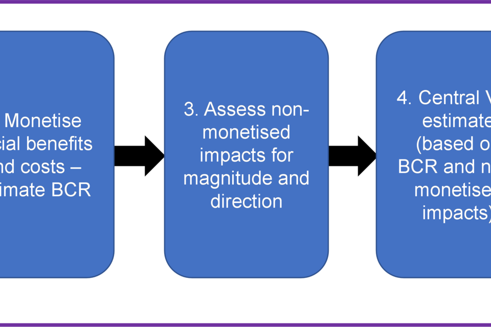
Develop evidence, options and narrative for a project.
Monetise social benefits and costs – estimate BCR.
Assess non-monetised impacts for magnitude and direction.
Central VfM estimate (based on BCR and non-monetised impacts).
VfM Category (based on sensitivity analysis and testing of assumptions.

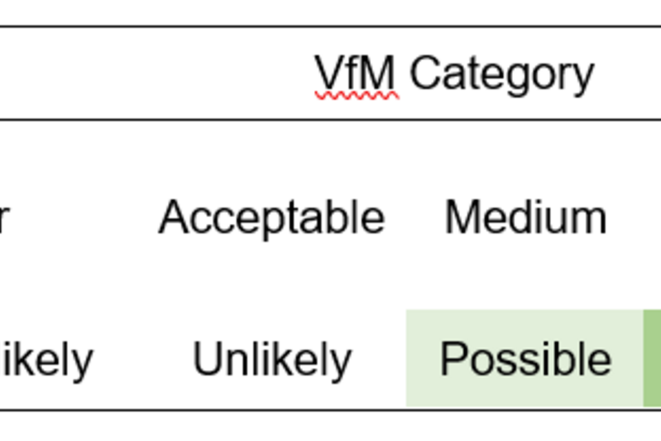
3.32 The following VfM categories can be defined where public sector costs are positive^{[footnote 19]}:

VfM Category	Implied by….
Very High	BCR greater than or equal to 4
High	BCR greater than or equal to 2 and less than 4
Medium	BCR greater than or equal to 1.5 and less than 2
Acceptable	BCR greater than or equal to 1 and less than 1.5
Poor	BCR greater than or equal to 0 and less than 1
Very Poor^{[footnote 20]}	BCR below 0

3.33 In the special case where the present value of costs is negative then the NPSV should be used alongside the categories in Annex I to define VfM.

3.34 As noted in the introduction to this section whilst the above bandings can be used to communicate the analysis, nothing should ever be described as VfM if it does not meet the policy objectives. Appraisal is a two-step process and all options that do not meet policy objectives must be filtered out at the longlist stage using the Options Framework, as per Green Book guidance.

Estimating VfM

3.35 To estimate VfM, monetised and non-monetised impacts need to be combined. The simplest approach to obtaining a central VfM estimate is to start with the BCR given by the monetised impacts and then ask the question:

How large do the non-monetised impacts have to be to shift the value for money of the policy to a different category, for example, from High to Medium (where the BCR is less than 2) or in the opposite direction from Medium to High?

3.36 The next stage is to assess all of the non-monetised impacts using the seven-point qualitative scale in Table 2 and ask the question:

Are any of the non-monetised impacts on their own or in combination large enough to shift the VfM category?

3.37 This requires:

The calculation of a switching value which shows how much benefits or disbenefits would have to change to shift the option to the next VfM category;
Comparison of the non-monetised impacts with the switching value to see if that size of change was likely.

A description of switching values is given in the Green Book (pages 52-54).

3.38 For example, suppose the BCR for a £10m investment is 0.9. It would require a £1m extra benefit to shift the BCR to 1 and for the investment to be categorised in a higher VfM category. Suppose there was a single non-monetised benefit and that it was assessed as being likely large so that it was likely greater than £1m. In this case the correct VfM category to use is Acceptable rather than Poor (which is what it would have been had only monetised impacts been considered).^{[footnote 21]}

Examining the impact of uncertainty on VfM

Types of uncertainty

3.39 In reality there is likely to be significant uncertainty associated with costs and benefits which may mean that a range of VfM categories rather than a single VfM category is the best assessment. For this reason, key uncertainties in the analysis should be explored and their impact on VfM assessed.

3.40 For monetised impacts uncertainty may arise from several different factors:

The degree to which an option has been fully defined, for example, the design of an investment is likely to be more uncertain at earlier business case stages;
The methods used to monetise impacts, in particular, the:
- Robustness of the measure used – for example, emerging measures used in the adjusted BCR are likely to have higher levels of uncertainty than those used for the Initial BCR;
- Models used to estimate impacts for a particular option can often take considerable time to fully develop or may be based on key assumptions which are subject to uncertainty. At early stages of analysis (for example the Strategic Outline Case) results may be subject to more uncertainty because the models are less developed;
- Some issues are inherently complex – perhaps involving multiple economic actors - so are more difficult to model;
- The evidence base underlying the theory of change may be less developed resulting in a lack of clear economic model to assess impacts;
The quality of data on which the modelling of options is based;
Uncertainty about the future and how it will impact on key variables (including input, output and outcome variables) and economic behaviour.

3.41 For non-monetised impacts there is inherent uncertainty caused by the inability to monetise the impacts.

3.42 There is a range of literature dealing with these issues. In particular, the Aqua Book sets out the importance of understanding uncertainty, developing robust models and ensuring that results are properly quality assured. The National Audit Office (NAO) reviewed how uncertainty is modelled, assessed and communicated across government and ways in which that can be improved (see Financial modelling in government and Why quality assurance is important in modelling). Both these documents should be read by the user to support the assessment of uncertainty.

Assessing uncertainty

3.43 Uncertainty in each of the elements set out in the previous section should be examined when drawing conclusions about the VfM of an option. This includes:

Identifying key uncertainties and risks in data, assumptions, models and the design of the options being developed;
Assessing whether they are likely to be significant; and
For significant areas of uncertainty, testing to understand the impact on VfM.

3.44 At a minimum, the impact of changes in key assumptions and inputs should be tested through sensitivity analysis. In particular:

Switching analysis should be used to assess how sensitive the VfM rating is to changes in costs and benefits.
For large schemes, where uncertainty may have a larger impact on the costs and/or benefits of a scheme, other techniques such as scenario or Monte Carlo analysis could be considered.^{[footnote 22]}
For more detailed guidance on how to handle uncertainty in appraisal including Monte Carlo and scenario modelling see the Uncertainty Toolkit for Analysts in Government.

Communicating VfM

3.45 It is essential that any approach and subsequent judgement is transparent and clear to decision makers when non-monetised impacts are considered to imply a different VfM category compared to the BCR alone. To make the judgement transparent, VfM categories and BCRs should be communicated in a Value for Money statement (which should be included with the relevant AST). A Value for Money statement will lay out what the estimated VfM category is and why this has been decided.

3.46 If the VfM rating is different from the BCR because of the existence of significant non-monetised impacts or a VfM range is adopted because of significant risk and uncertainty, the Value for Money statement will need to explain this.

3.47 As noted above a VfM rating may represent a range of VfM categories rather than a single category. The full range should be reported (for example Acceptable to Medium or Poor to Acceptable).

3.48 Where it is possible to allocate likelihoods to different VfM categories this should done. An example of how that might be presented is shown below.

3.49 Alongside an assessment of VfM it is important to be clear about the quality of the analysis. This should highlight any issues with the approach taken, whether there was enough time to do the analysis, fitness for purpose of the modelling, gaps in data or other significant risks to the conclusions of the analysis.

3.50 Three examples of how judgement has been used to inform a VfM category are set out in the Value for Money statements below.

Box 1: Examples of a value for money statement

Value for money statement example 1

The estimated value for money of this policy is Acceptable to Medium.

The costs of the policy are £100m. While the estimated ‘Adjusted’ BCR of this policy is 1.15 (implying Acceptable VFM) there is a potential for wider area impacts from the intervention which would have significant benefits. The switching value to move the VfM rating from Acceptable to Medium is £35m. The non-monetised impacts from wider area impacts are judged to have a reasonable probability of being greater than this.

The modelling that has been carried out quickly using high level modelling. Whilst it has been undertaken by experienced analysts there are concerns about the robustness of the approach. Consequently, the results need to be treated with some caution.

Value for money statement example 2

The estimated value for money of this policy is Medium to High.

The benefits of this policy are reduced CO2 emissions (central estimate equal to £10m) and increased land value (central estimate equal to £190m). The cost of the policy is the grant of £100m. There are no significant non-monetised impacts estimated for this policy.

The ‘initial’ and ‘adjusted’ BCR of 2 indicate there is £2 worth of benefits per £1 of net public expenditure.

There are some uncertainties around increased land value which could be less than £190 m if the local housing market slows. This would result in a fall in BCR below 2 and Medium VfM.

The modelling is robust using appropriate techniques and local data. It has been carried out and assured by analysts and reflects key uncertainties.

Value for money statement example 3

The estimated value for money of this option is Poor to Acceptable.

The costs of this option are £100m compared to benefits of £130m giving an adjusted BCR of 1.3 which would equate to a VfM category of Acceptable.

However, there are significant non-monetised biodiversity and landscape disbenefits. In addition, there is some uncertainty over costs which might rise to £120m.

For costs of £100m, biodiversity and landscape disbenefits of above £30m would change the VfM category to Poor. This is judged to be unlikely.
However, if costs rise to £120m then disbenefits need only rise by just over £10m for the BCR to fall below 1 and VfM to become Poor. This is judged possible.

The options being developed are at an early stage which is why some impacts have not been monetised. The analysis has been carried out quickly – although by experienced analysts – and there are likely to be large changes in results as options and modelling develop.

Externalities

3.51 An economic appraisal should seek to capture all the benefits and costs associated with an intervention. This will include both private and external impacts. In some cases, external impacts can be fundamental to the case for intervention.

3.52 Examples of externalities include: landscape and biodiversity impacts from reclaiming land or building on it; air quality and greenhouse gas emissions; transport impacts from new developments which might increase local road congestion; crime impacts because of changes in the environment (such as from better lighting); health impacts; and better educational outcomes from reduced overcrowding (see Annex G for more examples).

3.53 For the first time, estimates of wider area impacts in regeneration areas have been included in this Appraisal Guide and, where relevant, should be incorporated as part of the assessment of external impacts. Box 2 below provides a summary of wider area impacts and the work underlying them. Annex G provides a full overview of what is meant by wider area impacts and the methodology for calculating these.

Box 2: Wider area impacts

Wider area impacts refer to positive spill-over or external impacts from supply-side housing interventions with explicit placemaking and regeneration objectives resulting in the surrounding area becoming more desirable.

The guidance for the assessment draws on research commissioned by Homes England, based on a HM Treasury Green Book consistent hedonic pricing methodology, that examined the relationship between past Homes England interventions with placemaking objectives and post-intervention trends in house prices (over and above localised house price growth). The study found that, on average, regeneration supply-side housing projects are likely to have a positive wider ‘placemaking’ impact on the surrounding area, which can be measured based on net house price effects. Further analysis and spatial profiling enabled a methodology to be developed for assessing and monetising the wider area impacts of future projects.

The wider area impacts are applicable to supply-side housing interventions located within urban areas that have clear placemaking and regeneration objectives, which are likely to result in the surrounding area becoming more desirable. This should be clearly evidenced to the underlying rationale for intervention, the socio-economic and wider regeneration context and the objectives of the project as set out in the strategic dimension.

Wider area impacts are calculated based on estimating the uplift in the capital value of the surrounding housing stock, within a defined impact area, allowing for baseline trends and controlled variables to avoid double counting of other positive externalities. The modelled net rise in capital values implies a utility gain to local residents and reflects the increased willingness to pay of individuals for properties within the impact area, in the light of the improvements resulting from the scheme.

Given that this is a new methodology it should be included in the ‘adjusted’ BCR calculations.

3.54 The current version of the DLUHC Appraisal Guide provides estimates for the external amenity cost of development and the health benefits of additional affordable housing. Both the amenity cost of development and the health benefits of additional affordable housing should feature in the ‘adjusted’ BCR as these measures are evolving and there is some uncertainty around them. Some examples of how to deal with externalities are given below.

Box 3: Examples of externalities

Example 1: externalities are of second order importance

Assume there is a market failure which constrains the demand for housing (such as access to finance). Government intervention seeks to address this which leads to an increase in demand for new housing. As a result, additional houses are built and the monetised net private benefit associated with these additional houses - the additional land value uplift created - exceeds the public sector cost involved. While there are likely to be external impacts from such an intervention - such as reduced demands on health services because of better accommodation - these impacts are expected to be small in relation to the net private benefits and therefore they have little impact on the overall value for money assessment.

Example 2: externalities are important but not fundamental to the case

This could be similar to Example 1 with a similar market failure but instead the intervention ‘unlocks’ lower value development relative to the costs which results in a positive NPSV but a lower BCR. In this scenario, the economic case rests more strongly on the importance of wider impacts (externalities).

Example 3: externalities are fundamental to the economic case

In this example, assume that there is a potential development which generates an external benefit to society - perhaps there is an amenity and health benefit from developing a previously derelict site - but this development will not proceed without government intervention as there is insufficient private value. This is reflected in a Poor (less than one) ‘initial’ BCR. In this example, the value for money of the intervention relies on the significance of the externalities.

Natural capital

3.55 Where investments are likely to impact on natural capital including land, forests, biodiversity, fisheries, rivers or minerals then HMT green book supplementary guidance developed by the Department for Environment, Food and Rural Affairs (DEFRA) – Enabling a Natural Capital Approach (ENCA) – should be used to assess impacts.

3.56 Stocks of natural capital provide flows of environmental or ‘ecosystem’ services over time. These services, often in combination with other forms of capital (human, produced and social) produce a wide range of benefits.

3.57 These include use values that involve interaction with the resource and which can have a market value (minerals, timber, freshwater) or non-market value (such as outdoor recreation, landscape amenity).

3.58 They also include non-use values, such as the value people place on the existence of particular habitats or species.

3.59 To consider the impact of an intervention on natural capital the following questions should be asked. Is the option likely to affect, directly or indirectly:

The use or management of land, or landscape?
The atmosphere, including air quality, greenhouse gas emissions, noise levels or tranquillity?
An inland, coastal or marine water body?
Wildlife and/or wild vegetation, which are indicators of biodiversity?
The supply of natural raw materials, renewable and non-renewable, or the natural environment from which they are extracted?
Opportunities for recreation in the natural environment, including in urban areas?

3.60 If the answer to one or more of these questions is “yes” or “maybe”, further assessment is recommended using the following four steps:

Step 1: understand the environmental context to the proposal
Step 2: consider how natural assets might be affected
Step 3: consider the welfare implications, that is, how changes to the assets identified in Step 2 affect benefits provided to society by natural capital?
Step 4: consider uncertainties and optimise outcomes

3.61 DEFRA supplies templates for assessing each of these four steps.

3.62 Annex Giii of this document sets out estimates of the external amenity benefits associated with different land types. These estimates include values associated with recreation, landscape, ecology and tranquillity. These values can be used to estimate the loss of amenity benefits from development on different types of land.

3.63 Given the importance of Greenhouse Gases the next section discusses their estimation and valuation.

Greenhouse gases and climate change

3.64 Analysts should where possible quantify and appraise the impact of options on carbon emissions. Carbon emissions may arise for a number of reasons including:

Materials used in the development of sites and refurbishment of structures;
Transport of materials or changes in trip patterns from new residential or commercial sites;
Consumption of fossil fuels for heating, lighting or powering electrical appliances.

3.65 Some policies – such as better insulation or home generation of renewal energy – may reduce carbon. Newer buildings will generally be built to higher energy efficiency standards than older ones and it is important to factor in renewal of the building stock when assessing impacts.

3.66 Policy appraisal on climate change mitigation in DLUHC should use the Supplementary Green Book guidance on Valuation of energy use and greenhouse gas emissions for appraisal.

3.67 The guidance provides details on how to quantify and value energy use and emissions of greenhouse gases. It is intended to aid the assessment of proposals that have a direct impact on energy use and supply and those with an indirect impact through planning, land use change, construction or the introduction of new products that use energy.

3.68 It contains sections on:

Identifying the energy and emissions counterfactual and then policy interactions;
Quantifying and valuing changes in energy use and in emissions;
Identifying and quantifying other impacts, such as air quality; and
How to present findings and report for Carbon Budgets.

3.69 The guidance is accompanied by 19 data tables containing detailed estimates out to the year 2100 for carbon values and sensitivities, retail and long run energy prices, variable energy supply costs, and a GDP deflator. While the central estimates should be used in core analysis, care should be taken to reflect uncertainty in these estimates, for instance through sensitivity testing.

3.70 The guidance is updated regularly and so analysts should check that the latest version of the guidance is used in analysis.

3.71 For assessing how a policy / programme could be impacted by a changing climate, Supplementary Green Book Guidance on Accounting for the effects of climate change should be used. This supports the appraisal of policy options in the face of climate risks and uncertainty, and how adaptation of policies, programmes and projects can build resilience and enable flexibility in decision making.

3.72 The uncertainty over the future impacts of climate change and the importance of interconnections mean that climate resilience can prove important in unexpected areas of policy. Defra’s supplementary guidance supports analysts in identifying whether and how their appraisal should include climate risks.

3.73 There are other analytical challenges which help make appraising climate risk unique: thresholds and tipping points, long time horizons, the importance of early intervention, and lock-in. The guidance also supports analysts to address these challenges correctly.

3.74 In addition to levelling up and housing DLUHC leads on a number of the government’s major social programmes. These include the Supporting Families programme; policies to deal with homelessness, rough sleeping and domestic abuse; policies to encourage public service improvement, social cohesion and integration; and policies to improve the voting process and wider devolution issues.

3.75 Appraisal of social policies and public service improvement is based on the same principles contained in the Green Book but can present additional challenges, in particular estimating and monetising the net impact of redesigning services on the use of public services and wider economic and social outcomes. Detailed guidance on appraising public service improvement and social policies is set out in Supporting Public Service Transformation: cost benefit analysis for local partnerships.

3.76 Alongside this guidance, the Greater Manchester Combined Authority (GMCA) Research Team has developed a Unit Cost Database, to help with the appraisal of service transformation and social policies. Using the best available research from various government and academic sources, the database provides fiscal, economic, and social cost estimates for over 600 outcome measures covering a range of issues from crime, education, employment, fire, health, housing and social services. The database provides costs which can be used to monetise outcomes relevant to social policies in terms of costs to public services (fiscal costs) and the wider economy and society. The database is widely recognised across government as the best available source for information on the costs of a number of issues and is being extensively used for various appraisal projects across government departments and local authorities.

3.77 In addition to the guidance and the Unit Cost Database, the GMCA Research Team has also produced a model which acts as a template for carrying out cost benefit analysis.

3.78 Appraisal of Union, devolution and constitutional policies must incorporate place-based analysis where possible, as outlined in the updated Green Book and discussed in Chapter 5. This is essential in highlighting which areas and local authorities will be disproportionately impacted by the policies.

Question 7

4.  Land value uplift approach to appraising development

Accepted Answer

Introduction

4.1 The primary benefits of new residential and non-residential investments occur through land value uplift, where development increases the value of the land above its previous use, allowing for production costs.

4.2 This chapter introduces the concept of land value uplift, outlines how it might be calculated and used in cost benefit analysis, and how externalities and additionality are taken into account. The approach is also set out in DfT’s Transport Analysis Guidance (TAG).

4.3 A step-by-step guide for how to appraise residential development is given in Annex B and for non-residential development in Annex C. Annex D presents more detail on measuring additionality.

Land value uplift explained

4.4 Land value uplift, when used in appraisals, represents the private benefit, or change in economic efficiency, of one form of development on a particular site compared to its previous use. In a housing context, land value uplift is the value of land when used for housing minus the value of land in its current use. Generally, land value uplift will be higher where housing is of higher benefit to society, for example, in locations where housing supply is constrained relative to demand and/or where a site is near to local amenities or well-developed transport infrastructure. In short, the value of land is determined by a number of factors, but most significantly by its use and location.

4.5 The Gross Development Value (GDV) of a site is used in determining land values and therefore land value uplift. GDV is the estimated total revenue a developer could obtain from the land. In the context of housing, it would effectively be:

4.6 A developer will also incur costs and would expect a minimum level of profit from developing a site. The residual method of land valuation gives the maximum price a firm is willing to pay for the land. In a competitive market, the firm will pay a price that gives a normal level of profit. The land price is therefore equal to:^{[footnote 23]}

4.7 The uplift when land changes use is an estimate of the change, often increase, in economic efficiency arising from that change of use. In turn as discussed above this reflects the relative demand for and supply of land in its previous and new uses.

4.8 In an economic appraisal, analysts should seek to capture all costs and benefits of a policy. Costs should be economic costs and therefore capture the opportunity cost of the investment. For the developer investing money in the site results in foregone profits from investing the money elsewhere.^{[footnote 24]} This foregone profit is a cost and should be subtracted off the land price. Similarly wage costs reflect the opportunity cost of using labour in the development and should be subtracted off land price.

4.9 A simple example illustrates how land value uplift is calculated. Assume the economic value of land in its current use is low, for example, 50 owing to being an ex-industrial use brownfield site. Planning permission is then granted on that same site for a number of new homes. In its new use, assume the total obtainable revenue from the site is 300 (the GDV or sales revenue from the homes accruing to the developer), development costs to build the homes are 130 and the fees the developer occurs (such as legal fees, professional fees such as hiring quantity surveyors) are 30. Assume also that the market is competitive and that the level of normal profit is 40 – without this level of developer profit, the developer may instead choose not to develop this site and put their resources elsewhere. The new land value would then be:

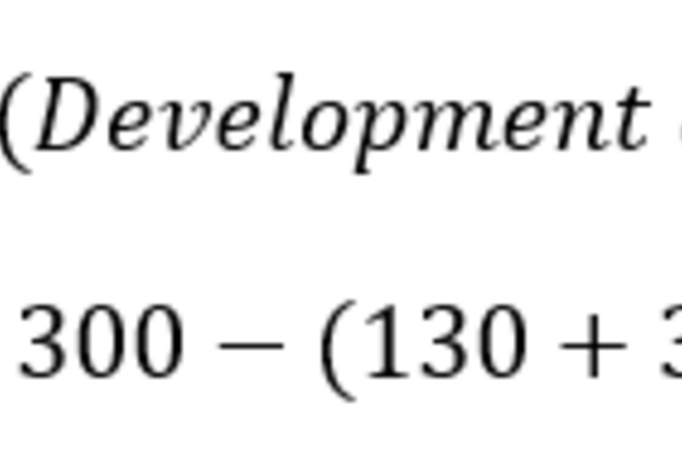
4.10 The developer is therefore willing to pay 100 for the land in order to earn a normal level of profit of 40. In an appraisal, the net private benefits from this development is therefore 50 (the land value in its new use, 100, less the land value in its previous use, 50).

4.11 The key point is that the land value is derived demand and means the land value includes the returns to all factors of production less economic costs, that is, returns to capital, land and labour (300) less construction costs (130) less fees (30) less expected profit (40). Therefore, changes in land values as a result of a change in land-use for a development reflect the economic efficiency benefits of converting land into a more productive use.^{[footnote 25]}

4.12 In practice some of the land value uplift is captured for the benefit of wider society through taxation and affordable housing requirements. If such obligations are included in developer costs or reflected in reduced income, they should be added to the land value as although they are a cost to the developer, they are a benefit to the recipient, such as for affordable housing.

4.13 Other planning obligations (Section 106, Section 278, CIL) can relate to both on-site and off-site infrastructure.

On-site infrastructure is often designed to benefit new residents and in such cases the benefit of this is likely to be captured already in the GDV of the proposals and so the land value uplift.
The purpose of off-site obligations is typically to mitigate for negative externalities caused by the development. In these circumstances, because the off-site obligation just removes the negative externality caused by the development, there would be no need to adjust the land value calculation.
However, on-site infrastructure may also benefit existing residents and off-site infrastructure could potentially provide wider societal benefits beyond mitigating for the negative externalities of development. Where this is the case and planning obligations have been included in developer costs, it may be appropriate to treat all or a proportion of these costs as additional transferred land value. The assumptions adopted in calculating this additional benefit must be clearly set out and justified.

4.14 Where local land value data is available, this should be used in the first instance to support land value uplift calculations. This could be informed by a site-specific development appraisal. Where this information is not available the VOA values published in DLUHC Land value estimates for policy appraisal can be used. These values do not assume any affordable housing. They also do not include any atypical costs or CIL, S106, S278 payments and need to be adjusted for these when used. In such cases ‘atypical’ private costs should feature as a negative number in the present value benefits as they represent a disbenefit to the private sector.

4.15 In summary:

Land price reflects the value of the land in its new use. In appraisal terms, the difference between this new value – once all costs of changing its use have been allowed for - and its previous value is the land value uplift and this represents the net private benefits of a development.
Land value data should be the primary means of assessing the private benefits of a development. Land value data is a rich source of information because it is actual market data on individuals’ / firms’ willingness to pay for a piece of land. Assuming individuals and firms are rational in their decision-making, market prices should reveal the ‘true’ private benefit of a development. This information can be used to undertake cost benefit analysis to quantify the potential welfare implications of a development.
Land value uplift is concerned purely with the net private benefits of a development (which accrue to the development’s new residents). External impacts – which affect existing residents of an area – should be accounted for separately and summed with the net private impacts to give the net social impact. See Annex G for a fuller discussion of the difference between private and external impacts.

Accounting for external impacts

4.16 Once the private benefits of a development have been calculated, external impacts should be assessed. The value to society of a change in use of the land may be separated into: (a) the private benefit associated with the change in land use, which is capitalised in the uplift in land value, and (b) the net external impact of the resulting development. The net social impact is then the summation of these two impacts.

4.17 The external impacts in (b) are in addition to the land value uplift. Examples of external impacts might include any amenity effects to existing residents of an area from changes in landscape or regeneration of the area. A full list is provided in Annex G. As explained in the externalities section, when accounting for externalities, the ‘initial’ BCR should be based on all impacts that can be robustly appraised using Green Book and Green Book Supplementary and Departmental guidance. The ‘adjusted’ BCR should then include a further range of externalities where the evidence base may not be as well established but which are important to consider in the overall appraisal. The ‘initial’ and ‘adjusted’ BCRs, non-monetised impacts and sensitivity analysis should inform the appropriate value for money category of the policy.

Using land value uplift in cost benefit analysis

4.18 Consider a hypothetical market for residential floor space (this example is also applicable to commercial floorspace). There is a supply curve S1 and demand curve D1 as per the diagram below.^{[footnote 26]}

4.19 The initial market equilibrium is where D1=S1, at which point price= P1 and quantity supplied=Q1. At this initial equilibrium point, the total market value of residential floor space is P1 x Q1 or A + E.

Figure 3: Supply and demand diagram for residential floor space

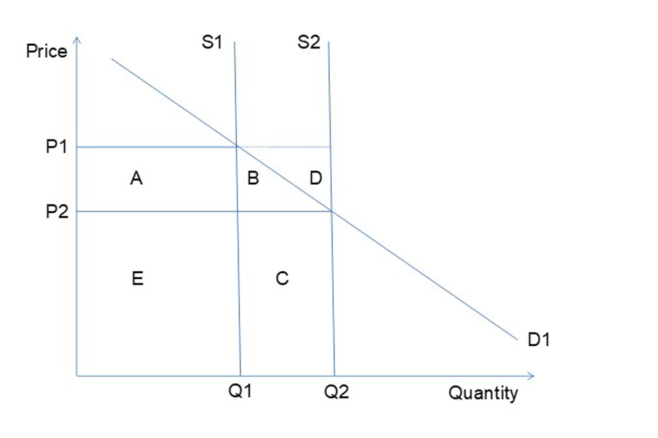
Figure 3 shows how consumer surplus changes as the supply of residential floorspace increases.

4.20 Assume government intervention is required to correct for a particular market failure which creates additional residential floor space (perhaps the government has provided financial support to ‘clean up’ a contaminated brownfield site thus correcting a negative externality). As a result of the intervention the supply curve shifts from S1 to S2. This results in a new market price of P2 and quantity supplied Q2. Consumer surplus^{[footnote 27]} increases by A+B while the total market value of the residential floor space is now P2 x Q2 or E + C (in other words the change in the total market value of the residential floor space is C - A). How this is then captured in an economic appraisal is discussed below.

Estimating the gross land value uplift impact from an intervention^{[footnote 28]}

4.21 A new development creates economic value which is reflected in the uplift of the value of the land. In this example, area C effectively measures the GDV of the development – the amount of residential floor space multiplied by the market price – so the land value uplift is equal to area C less development costs less profit less the value of the land in its previous use. This effectively goes to the existing land owners because land prices are bid up by developers.

4.22 For large changes in supply there are likely to be changes in the market price – shown as the reduction from P1 to P2 in figure 3. This leads to two other welfare impacts represented by A and B:

Area A shows a transfer of benefits from sellers to buyers of existing floorspace as a result of lower prices. The overall impact on welfare nets to zero.
Area B is additional consumer surplus that goes to ‘new’ buyers from being able to access the market at lower prices.^{[footnote 29]}

4.23 Many developments are local and small scale, so are likely to have a limited impact on the market price even within sub-national areas. In this case, Areas A and B are not counted when assessing welfare impacts. Where interventions are larger – particularly regional and national interventions – there may be some change in price. In this case Areas A and B need to be assessed. Larger scale developments are discussed in more detail in the section on displacement below.

4.24 Land Value Data for calculating Land Value Uplift (LVU) – In many instances, actual land value data may not be available and therefore illustrative values provided by the department can be used (these are explained in Annex B for residential development and Annex C for non-residential development). When using such values, the department would expect to see appropriate sensitivity analysis around these values to ensure a robust estimate of the (net) private benefit is made.

Estimating the net impact of an intervention

4.25 As Chapter 2 and Chapter 3 explain, all costs and benefits of an intervention should be compared against the business as usual counterfactual. The above example is based on a partial equilibrium analysis in the area where a development takes place. It therefore attempts to estimate the gross impact of an intervention. However, in a general equilibrium context, there are potential impacts that need to be considered in other markets / places. For example, as there will be development in the business as usual, it is important to account for the possibility that some of the benefits associated with this development would have happened anyway (deadweight) and that some benefits which would have occurred no longer do (displacement). Each of these is discussed below.

Estimating deadweight

4.26 Estimating the net impact of a policy requires any impacts which would have happened anyway to be subtracted from the gross estimates of a policy. In the example above, a critical issue is whether the expansion of floor space – and crucially the land value created – would have happened without government intervention, either in the location where the intervention takes place or somewhere else in the economy. In other words, ‘while an investment may be additional to the area in which it takes place, it may not be to a wider area or to the country as a whole’ (see Venables and others, 2014, page 45). Therefore, it is important that when appraising an intervention a correct counterfactual is established (see Chapter 2 and Annex D).

4.27 A key question to ask when trying to establish a counterfactual like the above is: why does the private sector require government support and would the private investment genuinely not happen without it? If there is a genuine market failure that means the development would not otherwise have happened without government support then there is no deadweight. It may also be the case that the development would have happened without government support but on a smaller scale, in which case there is some deadweight loss. Without a sound rationale for intervention (e.g. market failure), a high BCR consisting of mainly private impacts is potentially a sign of significant deadweight, that is, in the absence of the intervention the market would deliver the same outcomes. In this instance, it would be appropriate to revisit the additionality assumptions underlying the BCR calculation.

4.28 In some instances, it may only be appropriate to include the external impact of a development – such as the positive external (amenity) value of redeveloping a previously derelict site or wider area regeneration impacts – in the additional economic benefits because the development would have gone ahead somewhere in the country but not necessarily on a brownfield site. Strategic considerations will be important in determining this. For example, the clustering of economic activity of a particular sector in a particular area may mean a firm is unlikely to want to locate somewhere else (see Annex D).

Estimating displacement

4.29 As well as potential deadweight, some developments will result in economic activity being displaced from one location to another. An appraisal should seek to capture the gross impact of a development (as measured by the land value uplift) and deduct any reduction in economic activity elsewhere from displaced activity (as well as any deadweight). This will give the net change in land value (or overall additionality).

4.30 There are various ways to take displacement into account. The level of assessment should be proportionate to the scale of the intervention.^{[footnote 30]}

4.31 Smaller scale interventions – where the constant price assumption holds – should follow the detailed approach set out in Annex D.

4.32 Larger scale interventions are likely to require additional analysis:

For interventions large enough to result in changes in prices at the local level but not regionally the land value uplift should be adjusted down. An assessment of impacts on land value uplift for other planned developments in the local area should also be made. Effectively this means calculating an ‘additionality factor’ across the local area;
For very large interventions which are likely to have significant regional impacts a structural economy model could be used to examine impacts including:
- The total change in land prices for new developments across all areas; and
- The spatial and sectoral distribution of economic activity.

4.33 Structural economy models have different strengths and limitations and can take time to set up and run effectively so the choice of which to use should be made carefully.^{[footnote 31]} When these models are being used it is very important to state assumptions, be clear about key uncertainties and carry out sensitivity testing around key parameters.

Distributional considerations

4.34 As noted above, large developments are likely to result in changes in the price of residential and non-residential property. These changes in price will have distributional implications:

In a housing context, the release of new land for development reduces the scarcity of residential land, and so reduces the value of existing residential land. This reduction in value should be regarded as having purely distributional effects – there is a transfer from the asset-rich who lose out from new development, to the asset-poor, including non-homeowners, who gain.
The economic benefit of expanding non-residential space is captured by existing companies that use that space in the form of rents being lower than they otherwise would have been. Income is thus transferred from existing owners of the floorspace to users of the floorspace (see Venables and others, 2014, page 48).

4.35 If Figure 3 was to be applied separately to both residential and non-residential floorspace, the size of the distributional transfer in both cases would be equal to area A.

4.36 However, any additional (gross) land value generated by new development (Q2-Q1 in Figure 3) is not a transfer as the land has been developed into a more productive use.^{[footnote 32]}

Other issues to consider

4.37 Any private costs associated with the development should be included in the appraisal as a disbenefit and therefore feature in the numerator of the BCR calculation (unless such costs have already been accounted for in the residual land value estimate (see the BCR section for further details)). All public sector costs should also be included and feature in the denominator of the BCR.

4.38 When carrying out an appraisal it is essential that there is no double counting of impacts. This could be an issue where local land value data is used. Land value data captures the full net private benefit of a change in land value. For example, any utility derived from being close to open space may be reflected in the value of the land. For non-residential interventions too, in theory, the full private (commercial) benefit of a development will be reflected in the land value, though there may be an external impact on others such as through agglomeration impacts (see Annex G).^{[footnote 33]}

Question 8

5.  The appraisal of place based initiatives

Accepted Answer

Introduction

5.1 Appraisal of place based impacts is particularly important for DLUHC Levelling Up Policies. Levelling up involves reducing spatial inequalities and raising opportunities in left behind areas through:

Raising productivity, pay, jobs and living standards in those areas;
Improving education, skills, health, and wellbeing;
Improving the sense of community by developing pride in place, improving housing and reducing crime; and
Empowering local leaders and communities through devolving powers to the local and regional level.

5.2 The Levelling Up White Paper identified six key capitals which together likely explain much of the disparity in economic performance across geographies:

Physical capital – infrastructure, machines and housing;
Human capital – the skills, health and experience of the workforce;
Intangible capital – innovation, ideas and patents;
Financial capital – resources supporting the financing of companies;
Social capital – the strength of communities, relationships and trust;
Institutional capital – local leadership, capacity and capability.

5.3 Low levels of capital formation in specific geographies – often in multiple sectors – lead to underperformance relative to the UK economy as a whole. These capitals are interrelated, with sustained feedback loops, so that a fall in the stock of one type of capital impacts on others. Left behind areas will often face multiple capital shortfalls.

5.4 Within this levelling up context effective appraisal must be able to:

a. Provide policy makers with an understanding of how policy options impact on local areas, regions and different groups; and

b. Deal with multiple and complex interventions covering a range of different issues caused by low levels of capital formation.

Chapter aims

5.5 This chapter aims to show how:

To appraise place based initiatives so that informed decisions can be made on which policies to pursue to achieve levelling up objectives; and
Multiple policies can be appraised together to reach a single view on their costs and benefits.

5.6 The chapter builds on Annex A2 of the Green Book which includes a new expectation that appraisals assess the likelihood and extent of differential place based impacts. Place based analysis will be needed when either:

a. The objective of the proposal is aimed at a particular place, area or type of area; or

b. The proposal is likely to have different impacts on different areas.

Structure

5.7 This chapter is structured in the following way:

The next section discusses the role of place based analysis in appraisal and sets out the key analytical questions to ask when assessing interventions aimed at levelling up places or which have a significant impact on those places. The section makes clear that to adequately appraise impacts there needs to be a strong focus on place and the people in the place.
The following section discusses some key issues when appraising place based interventions – including the relationship between strategic objectives and social welfare, the assessment of employment impacts and the importance of understanding wellbeing impacts.
The penultimate section presents an illustrative example of place based analysis using a hypothetical intervention covering labour market, business support, housing and transport interventions. The section provides an example of how to respond to the key questions defined for the strategic and economic dimensions of business cases in the next section.
The final section identifies some areas where it is intended to develop both place based and levelling up analysis.

The role of place based analysis in appraisal

5.8 The Green Book says that where a proposal has geographically defined objectives, then place based analysis can be the primary frame of reference for appraisal. This should be supplemented with UK level appraisal or analysis wherever possible:

Place based analysis may involve consideration of local employment effects, distributional impacts on demographic/protected groups and on intervention target groups.
It should be based on a robust understanding of local conditions, constraints and plans and consider both the positive and negative impacts of policy options.

5.9 Place based analysis where it is applied to business cases is likely to form a key element of the:

Strategic Dimension – setting out the place based nature of the problem that needs to be dealt with, and key place based objectives;
Economic Dimension – looking at the economic impacts across different areas and groups; and
Management Dimension – showing how place based effects will be monitored and evaluated.

5.10 Place based analysis may also be important for the:

Financial Dimension – where income is raised locally; and
Commercial Dimension – where there is a focus on the local market to deliver the services set out in the business case.

5.11 What follows concentrates only on the strategic and economic dimensions as they are the main focus of appraisal. However, the importance in the management dimension of having an appropriate evaluation framework that allows identification of place based impacts and place based metrics to monitor performance should be emphasised.

Proportionality

5.12 The degree of analysis should depend on the relative importance of the programme (e.g. the amount of money involved), the degree of importance attached to local outcomes and whether there are any key local delivery risks.

Robustness of analysis

5.13 Local data and models constructed for specific one-off purposes may be less developed than nationally available data sets or long standing models. For this reason, it is important throughout the analysis to report on the robustness of the modelling and data used in any place based analysis.

Key questions

5.14 The following key questions could be used to support the development of place based appraisal. These have been separated into questions that could be posed in the strategic dimension and the economic dimension of a business case, respectively:

a) Strategic dimension

1. What are the key issues that are being addressed by the policy? To what extent do those reflect issues in specific places, areas or types of area?

2. What are the key spatially focused objectives which address the issues above that options must look to satisfy?

3. What do the different options look like spatially? What does the preferred option look like compared to the counterfactual and what is its spatial coverage? To what extent is it focused on specific places, areas or people?

4. What is the spatial impact of the intervention:

On specific places, areas or people?
On the UK as a whole?

For this careful consideration needs to be given of any shift in activity between the area of focus and the rest of the UK, such as employment.

5. What are the key local risks that might impact on the delivery of a policy at local level?

b) Economic dimension

6. What are the costs and benefits of the leading intervention:

On specific places, areas or people?
On the UK economy?

Where firms shift economic activity from one area to another the impacts on the area from which they move need to be understood too and the degree to which that is beneficial or not, for example if the shift is from an area of greater economic need.

7. How has additionality been assessed in particular:

Deadweight – what would have happened in the absence of the intervention;
Substitution – where firms substitute one type of labour for another to benefit from an intervention;
Displacement – where outputs shift from firms not benefiting from an intervention to those that benefit from it;
Leakage – the impacts leaking out of the target area or target group (if the aim is to improve prospects for certain people, e.g. low skills/disabled).

8. How does the intervention impact on different target groups, for example:

Local residents versus commuters or people moving in;
Different income (e.g. age, need) groups; and
Employment impacts if it is thought that there are any.

9. What are the key uncertainties and what is their implication for impacts and VfM?

5.15 Where possible maps should be used to demonstrate problems, set out how interventions would work and to look at the impact on people.

Issues in appraising place based initiatives

5.16 Place based appraisal involves assessing two key separate but related criteria:

The achievement of strategic policy objectives – these may be local objectives or national objectives which have a local impact. This explicitly comes into the strategic dimension.
Social Welfare from pursuing a particular option linked to the policy. This explicitly comes into the economic dimension^{[footnote 34]}.

5.17 The strategic objectives a policy pursues will generally be linked to social welfare but need not necessarily be exactly the same. For example, a key objective may be to raise the level of output in an area or to raise the level of employment. These objectives are related to social welfare but not the same generally.

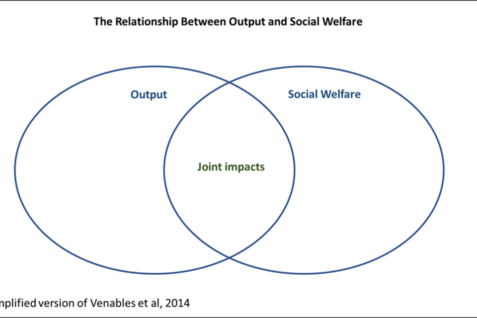
An output circle and a social welfare circle overlapping. It shows that they are different concepts although there is some overlap.

Economic output

5.18 Economic output ignores a number of factors that enter into social welfare:

Although the value of what workers produce is included in output as the wages paid to them (reflecting their productivity), the social welfare that workers receive from the job will be different because they have to give up leisure to work (a disbenefit) and receive personal wellbeing from being in employment (a benefit). Evidence from the 2021 supplementary guidance on valuing wellbeing indicates that the overall impact of being in work (after income, health and other standard factors have been allowed for) is positive, with a central value of £5,980 per annum in 2019 prices. This means the market value of their output is less than their social welfare from employment. If there are net employment impacts then wellbeing impacts need to be taken into account when assessing social welfare in the economic dimension;
Some things are excluded from economic output which impact on social welfare measures. Important examples of these are:
- Environmental impacts such as amenity, noise and pollution impacts (including carbon impacts);
- Social impacts such as on crime levels and health from changes in the physical environment;
- Community wellbeing impacts which spillover from individual impacts and reflect greater social cohesion and greater levels of optimism; and
- Any costs to workers of getting to work, such as the value of time and uncertainty caused by congestion and reliability issues.

Many of these impacts can be monetised and included in BCRs (see Annex A1 of the Green Book).

5.19 However some types of impact are included in both social welfare and economic output measures. These include Land Value Uplift, increases in productivity as a result of skills policies or economic agglomeration and taxes on economic production (e.g. labour taxes).

5.20 Given that some impacts do not impact on social welfare they are better left to the Strategic Dimension than to the Economic Dimension. This does not mean that they are excluded from the decision on which option to select as all options must meet strategic objectives. Rather, it reflects a need to account for impacts in the right place.

Employment

5.21 Increasing local employment is often a key strategic objective of place based initiatives. In line with HM Treasury’s Green Book the default assumption is that any jobs created by a policy resulting from government expenditure do not increase aggregate UK employment as these employment effects are already largely determined by macroeconomic decisions on the level of overall public expenditure (though they may have an important local impact). However, if there is a supply side impact which raises overall productivity or increases entry into the labour force (once additionality has been allowed for) these impacts can be counted at the UK level in the appraisal.

5.22 It is, however, permissible to include local labour demand effects in place based analysis where an intervention has geographically targeted employment objectives. Where levelling up is concerned, then regional and local employment effects may form a key part of the analysis and, if so, should be considered.

5.23 When considering employment effects the analysis needs to allow for:

Deadweight – what would have happened in the absence of the intervention;
Substitution – where firms substitute one type of labour for another to benefit from an intervention;
Displacement – where outputs shift from firms not benefiting from an intervention to those that benefit from it; and
Leakage – the impacts leaking out of the target area or target group (if the aim is to improve prospects for certain people, e.g. low skills/disabled).

5.24 The analysis may also take account of multiplier effects. The appropriate multipliers to use will depend on the local labour market and the sector in which employment changes. Where the employment rate is at or above the national average and/or projected local employment numbers are large relative to the local unemployment rate, multipliers at the lower end of the range would be expected as the likely level of displacement will be greater.

5.25 The illustrative example in the next section includes a discussion of employment impacts and allows for deadweight, substitution, displacement, leakage and the application of multiplier impacts. It shows how employment impacts are reported in the strategic dimension of a business case and how to report the welfare impacts associated with changes in employment across areas in the economic dimension. In the illustrative example demand impacts net to zero across areas in line with HM Treasury guidance, however supply side impacts are positive. Further detail on how to estimate employment impacts, including a detailed worked through example, is presented in Annex 2, Box 27 of the Green Book.

Range of impacts covered by levelling up policies

5.26 The Levelling Up White Paper covers a wide range of policy areas and impacts. The appraisal of many of these policy impacts is covered by other departments’ supplementary guidance. A summary of the types of impacts on which other departments offer guidance is set out in Annex A1 of the HM Treasury Green Book and users should consult it for the appraisal of impacts not covered in this guide.

An illustrative example of place based analysis

5.27 This section sets out an example of how place based analysis might be conducted by answering the different questions set out in the previous section. The example is purely illustrative, and the case study area does not relate to any existing administrative boundary.

5.28 The example covers a complex programme of interventions on purpose to show how these might be dealt with together. In practice many interventions are likely to have a simpler structure. A proportionate approach to the analysis should be adopted. Smaller, less expensive interventions with lower levels of risk should adopt a proportionate approach to monetisation.

a) Strategic dimension

The key issues that are being addressed by the policy

5.29 The example relates to Place A – a left behind area. Place A experiences significant deprivation caused by high levels of structural unemployment with unemployed workers lacking the skills needed by local industry. Most workers are employed in low skilled jobs. Much of the industrial and commercial business area is derelict or underutilised. There is significant blight from dereliction, some of the industrial land is contaminated and requires remediating before it can be used again. Residents experience poor health outcomes and wellbeing from low levels of social capital. Place A faces high demand for public services but local resources needed to meet those demands are limited because of the low tax base. It is difficult for Place A to attract new business to the area because of the problems the area faces.

The map below shows the existing area before the intervention

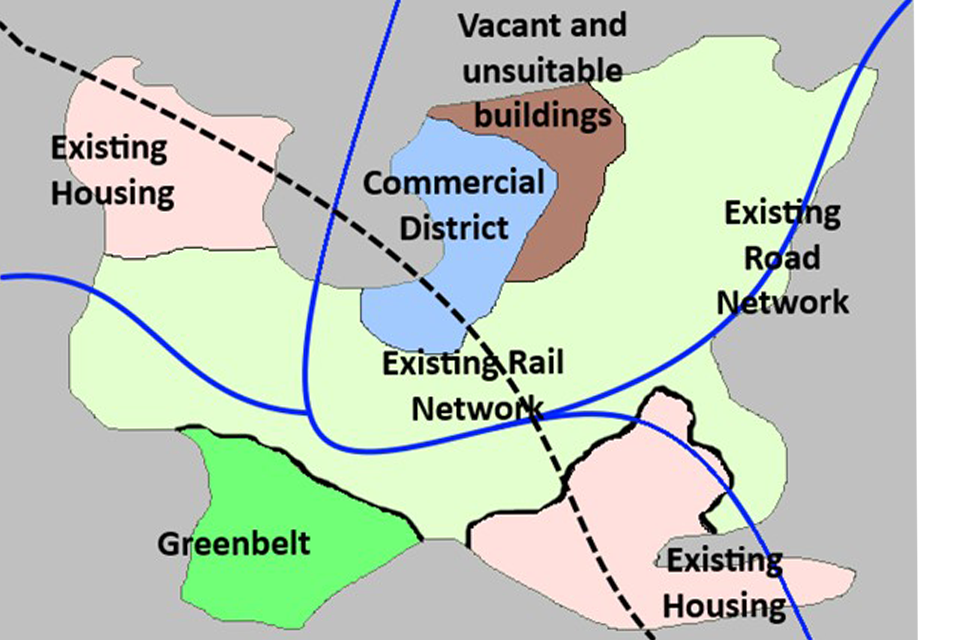
Rationale for investment

5.30. Without government intervention Place A is likely to remain a left behind area. This is because:

Local unemployed and low skilled workers do not have the resources to retrain - there is a credit constraint;
Blight makes the area unattractive to developers and to new business; and
The complexity of the problem to be dealt with creates a co-ordination problem which will not be solved if left to itself.

Key objectives for the intervention

5.31 The key local objectives are to improve economic outcomes for local residents by:

Increasing the number of jobs for residents in Place A area over the next five years and thereby reducing levels of unemployment – particularly long-term unemployment – towards UK national averages;
Increasing the level of skills of the local workforce so that wages will increase to UK national average levels over the next five years;
Regenerating the local area by redevelopment and removal of blight over the next two years;
Attracting high skilled firms to the local area so that overall productivity and output increases over the next five years to the UK average; and
Improving the level of wellbeing in the area through creating more positive outcomes for local people over the next five years.

5.32 The chosen option must also meet wider Critical Success Factors (see Box 9 of the HM Treasury Green Book) in particular, it must:

Provide Value for Money – so that social benefits exceed costs nationally;
Be affordable – money must be available to fund the option;
Be commercially viable – so that suppliers are able and willing to deliver relevant elements of the chosen option; and
Be achievable – both in terms of implementing the programme and delivering key objectives.

Description of the options considered and spatial coverage of the preferred option

5.33 A number of options have been considered including the following:

Business As Usual – continue as is with no intervention;
Preferred Way Forward (PWF) – this involves several intervention strands, for example:

Strand 1 – Redevelopment of 25,000 sq. metres of commercial space and 2,000 homes, including removal of blight from the local area. Costs £35m over two years;

Strand 2 – A new road to support access to the redeveloped site. Costs £30m over two years;

Strand 3 – £22m over five years for the provision of skills training to:

Help local long-term unemployed workers get into work; and
Offer an apprenticeship scheme for low skilled workers to raise their productivity and make the area more attractive to new firms.

Strand 4 – Business tax rate reductions in Place A over a period of 5 years to attract new business. The estimated public sector cost is £10m;

Strand 5 – Business support to local firms to make them more competitive by supporting innovation. Costs £4m over five years;

Strand 6 – Community involvement in the design of the programme to make sure it meets local needs. Costs £2m over five years.

Do Minimum – A less ambitious version of the preferred option. This might involve redevelopment of a smaller area and skills training for a smaller number of people.
Ambitious PWF – A more ambitious version of the preferred option. This might involve widening the scope of the intervention to include additional incentives for businesses to locate to the area.

5.34. In the example that follows only the preferred option is compared relative to the BAU to save space.

The map below shows the new infrastructure interventions in the area

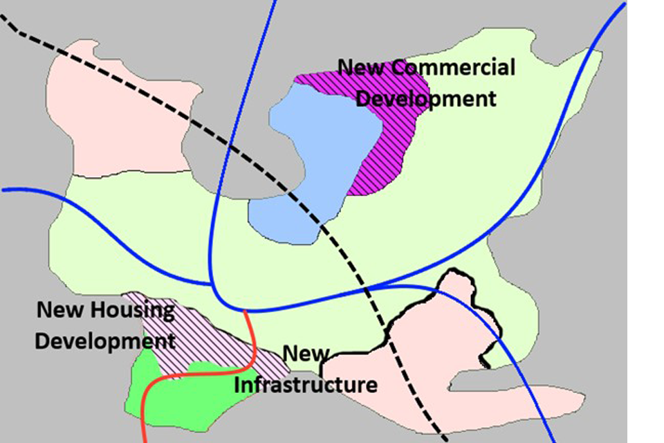
The spatial impact of the preferred option on key objectives:

5.35 Jobs – By Year 5, the initiative will result in 740 new jobs for local residents (see chart 1). New jobs come from three sources:

Improving the skills of the long-term unemployed and unskilled workers;
Attracting new firms to Place A who employ local residents; and
Indirect multiplier employment effects in traded and non-traded sections.

5.36 Increased competitiveness through better business support may also raise the level of employment amongst residents.

5.37 Although local employment effects are significant, national effects are somewhat smaller. In particular, it is assumed that jobs that go to local workers as a result of firms relocating are all displaced from other areas in the rest of the UK. Similarly, there will be negative multiplier effects in other areas from displacement. For this reason the rest of the UK experiences a fall in the level of employment. (It should be noted that allowance has been made for the fact that some employment will go to commuters who live outside Place A but work in it.)

5.38 The rest of UK and national impacts on employment over the 5 years covered by the strategic objective are shown in chart 1 below. The rest of the UK impact partially offsets Place A’s impact.

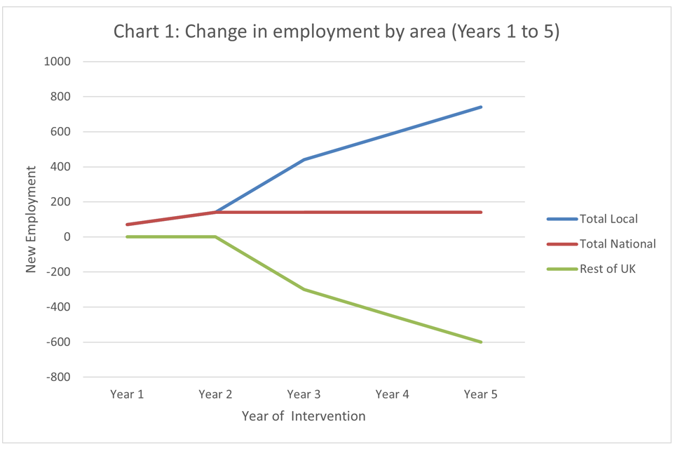
Productivity and skills

5.39 Approximately 500 people will complete level 2 apprenticeship training and move into higher skilled jobs. In this illustrative example, the wage increase is assumed to be £10,000 per worker per annum.

5.40 There are also likely to be a general increase in productivity from the business support programme which is focused on innovative training. Finally there will be a general increase in productivity for the area from agglomeration impacts, although these will be offset to some extent from disagglomeration impacts in the rest of the UK.^{[footnote 35]}

Regeneration of the local area

5.41 The redevelopment will result in the removal of 15,000 m2 of substandard buildings and its replacement with 25,000 m2 of commercial space and 2,000 houses. In addition, the surrounding area which is subject to blight will be landscaped and turned into a park. There are likely to be significant positive impacts to existing residents from the improved local environment.

Improved wellbeing

Increased access to employment is likely to significantly improve wellbeing. As noted above the 2021 Wellbeing Guidance for Appraisal indicates that a worker who has a job receives a wellbeing effect of nearly £6,000 a year (in 2019 prices). This is assessed in the economic dimension appraisal;
Similarly access to better quality jobs for workers who have gone through apprenticeships is likely to raise wellbeing, as will the improved environment and greater social cohesion;
Increased income for low income workers may also improve health outcomes which raises wellbeing;
There will be an increase in positive outcomes in the area generally which will improve the level of wellbeing for local residents; and
Finally it should be noted that some of these impacts are likely to be offset nationally (e.g. displacement of jobs will reduce wellbeing in other areas).

Social and institutional capital

5.42 Under the preferred option:

The local community will be involved in the design of the redevelopment and in the labour market programme aimed at tackling unemployment and low skills;
Similarly local businesses will also be involved in the design of the overall programme;
The programme will be led by the LA in Place A and will involve input from other key public sector partners; and
Post implementation there will be a local governance forum with the responsibility of overseeing the implementation the programme.

5.43 As a result of all the actions above the programme will support the development of a stronger community identity and pride in place.

Key risks that might impact on the delivery of a policy

5.44 Five major risks are identified in this illustrative example:

i. Commercial and residential values and consequently land value uplift might be lower than estimated because of adverse local economic conditions – this is assessed through sensitivity tests;

ii. Costs of the project might be higher than anticipated – this is dealt with in the economic dimension through the application of optimism bias and cost sensitivity tests;

iii. Failure to adequately target the employment based initiatives on those who need the initiative most – this is dealt with by involving local community in design of programme and active programme monitoring;

iv. Failure to engage properly with the local community resulting in poor design of the programme and lower levels of effectiveness and community wellbeing – this is dealt with through active stakeholder engagement in design and implementation of the option; and

v. The valuation of wellbeing benefits may be too optimistic – this is mitigated by carrying out a sensitivity test with a lower well-being value.

b) Economic dimension

Assumptions used to calculate costs and benefits of the leading intervention

5.45. Costs and benefits are calculated over the relative lifetime of the different interventions. All costs and benefits in this illustrative example are valued in current year present value terms.

5.46 Table 3 provides a breakdown of monetised and non-monetised impacts for relevant costs and benefits. All impacts are measured relative to the business as usual counterfactual (that is they take account of deadweight). Some grouping of impacts has been done to simplify presentation. Only large and medium scale non-monetised impacts are reported as only these are likely to influence the VfM assessment.

5.47 In this illustrative example costs and benefits are reported for Place A (the local area of interest), for the rest of the UK and at UK level. (This approach could easily be extended to further spatial tiering, for example, multiple LAs, region and UK level.)

Where possible, relevant impacts should be estimated in line with appropriate departmental guidance. For example, transport benefits would require a transport model and use DfT guidance, carbon impacts would use Department for Energy Security and Net Zero guidance, and Wellbeing estimation would use the relevant supplementary guidance.
The illustrative figures represent central assumption estimates.
For employment and wage impacts of people with low incomes, distributional weights have been applied in line with Annex H of this guidance.

Additionality

5.48 In addition to allowing for deadweight, full allowance is made for:

Substitution of existing workers with unemployed workers who are going through the apprenticeship training scheme – it is assumed that 20% of apprenticeship jobs displace existing workers;
Displacement – some economic activity which occurs in Place A is likely to displace activity outside of the area. In particular the following sectors are likely to be impacted:
- Commercial and housing – 25% displacement after applying the additionality guidance in Annex D;
- Benefits from employment – all jobs that move to Place A from outside result in a net zero effect across the UK, that is, they are displaced. Multiplier impacts for these jobs also represent displacement between rest of UK and Place A.
Leakage – is allowed for with 10% of new employment jobs being filled by commuters into Place A (based on existing travel to work statistics). Note that skills and unemployed worker programmes are targeted on Place A residents and impacts take place within the area.

Estimated costs and benefits of the leading intervention

5.49 Overall the total present value of monetised benefits for Place A in this illustrative example are £334m. The major impacts are from:

Land Value Uplift as a result of commercial and residential redevelopment and associated regeneration of the area from removing blight and improving landscape;
Employment benefits from enabling unemployed workers to get jobs through improving their skills. This results in increased income to them and welfare gains from having a job, as well as employment tax benefits to the UK government (not shown separately);
Wage gains to workers whose skills increase and to the exchequer from increased taxes;
Employment benefits to local workers as a result of firms shifting location to Place A from the rest of the UK. This results in income and employment tax benefits. There are also employment multiplier impacts; and
There are also some transport benefits from the creation of a new link road to the commercial site and improved journey time reliability.

5.50 For the rest of the UK the picture is much less positive. In particular:

There will be some employment losses because of displacement;
Similarly some of the commercial development in Place A will crowd out other development;
Welfare impacts will be negative because of reduced employment; and
This emphasises the importance of understanding displacement effects and the impact on the rest of the economy.

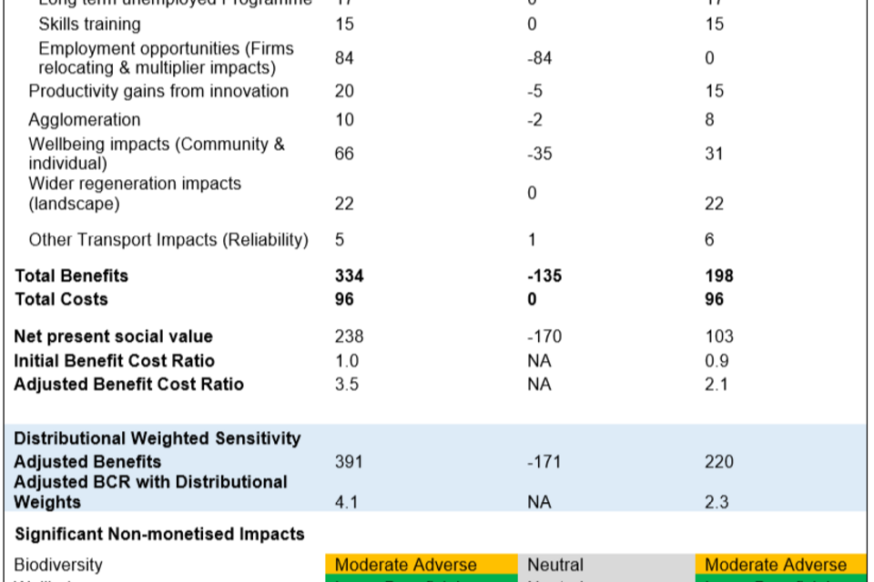
Overall value for money of the preferred option

5.51 Two measures of VfM are assessed:

VfM to Place A – reflecting the fact that the programme of interventions is focused on Place A;
VfM to the UK economy – reflecting the fact that the programme should yield more for the UK taxpayer than it costs (that is BCR>1 allowing for non-monetised impacts).

5.52 In this illustrative example:

The overall BCR for the UK is 2.1, so that the programme yields over £2 of benefit per £1 spent.
The impact on Place A is £3.5 of benefit per £1 spent which is higher, reflecting the transfer of employment from residents in the rest of the UK to residents in Place A.
Non-monetised impacts are on balance positive, with large beneficial wellbeing impacts and moderate crime and health impacts outweighing moderate adverse biodiversity impacts.
For Place A the overall conclusion is that the VfM of the project is Very High. However, the VfM rating falls to High for the UK as a whole.

Distributional impacts

5.53 The blue lines in Table 3 allow for distributional impacts from applying the welfare weights in Annex H to unemployed and low skilled workers who benefit from the investment package. Doing this results in an increase in benefits within Place A to £391m and increases the Adjusted BCR to 4.1. The UK BCR increases to 2.3. The overall effect of applying distributional weights in this particular illustrative example is to confirm the assessment of the investment package as representing Very High VfM for Place A and High VfM for the UK.

The impact of the preferred option on different target groups

5.54 The target groups picked in Table 4 include those covered by the policy objectives and protected groups and are shown below. Overall, the impacts tend to be positive on target and protected groups supporting further the choice of the preferred option in this illustrative example.

Table 4: Impact of option on different groups

Group	Impact	Commentary
Local Community	Positive	Option aimed at supporting better outcomes for local residents through lowering unemployment, increasing wages and improving local wellbeing.
Long-term Unemployed	Positive	Tailored programme increases job opportunities for long-term unemployed.
Age	Positive	Positive for 16-24 through increased apprenticeships and for older workers as many unemployed are over 50.
Gender reassignment	Neutral	No distinction in application of option made on basis of gender reassignment.
Sex	Positive	Option applied equally to different sexes.
Being married or in a civil partnership	Neutral	Marital status not a feature of the option.
Being pregnant or on maternity leave	Positive	Support given to access programmes.
Disability	Positive	Support given to access programmes.
Race including colour, nationality, ethnic or national origin	Positive	Support given to access programmes.
Religion or belief	Neutral	Religious belief not a feature of the option.

Key risks and the impact of their crystallisation on VfM

5.55 The impact of the crystallisation of the five key risks identified above is analysed in Table 5 below. The probability of these risks occurring is shown on the right assuming that all possible mitigation procedures have been put in place. This is assumed to be based on a thorough analysis of the evidence on risks by the programme team.

Table 5: Impact of five different risks on the VfM of the Preferred Option

	Place A - BCR	Place A - VfM	UK - BCR	UK - VfM	Probability of risk occurring
Commercial and Residential Land Values 15% lower	3.37	High	1.99	High	Medium
Costs of Redevelopment increase by 50%	2.64	High	1.57	Medium	Medium
Costs of Redevelopment reduce by 50%	5.13	Very High	3.05	High	Low
Employment/skills training 20% less effective than planned	3.34	High	1.93	High	Medium
Failure to engage with local community	3.19	High	1.78	High	Low
Wellbeing Value Low range	3.36	High	2.01	High	Medium

5.56 In this example, the preferred option provides at least Medium VfM under all options and consequently is relatively robust to risk challenges.

Further analytical research

Understanding future needs

5.57 Analysis of placed based impacts is still at an early stage. Further work is being done to:

Develop the measurement of the six different capitals and assess levels of need in different local areas;
Look at how shortfalls in different capital levels interact and impact local economic performance, and what mixtures of programmes best address those shortfalls.

5.58 Research in these areas will be incorporated in future levelling up guidance.

Transformational impacts

5.59 In some cases, transformational change programmes may be required to level up the area where there are shortfalls across multiple capitals.

5.60 Annex A7 of the HM Treasury Green Book defines transformational change as:

A radical permanent qualitative change in the subject being transformed, so that the subject when transformed has very different properties and behaves or operates in a different way.

It refers to a “practically irreversible change in a system” that causes self-sustaining internal feedback effects that result in continuing change, or a new stable state, but not reversion to the original state. This transformation persists after the initial stimulus is withdrawn.

5.61 Such change is only likely to occur in areas where there are multiple capital deficiencies and they are of significant magnitude. The achievement of transformational change will require all of those deficiencies to be addressed. Consequently, strategic investment portfolios will likely be required, rather than single interventions, even if those interventions are of significant scale. The area of intervention needs to reflect adequately the level of need.

5.62 The issue of how to assess transformational change is one where there is currently limited consensus or evidence. This is an issue that DLUHC is actively seeking to explore going forward and to eventually incorporate into further guidance. This will build on this appraisal guidance on Annex A7 of the HMT Green Book by looking at:

Developing appraisal approaches to assess large scale, multi-dimensional programmes and portfolios of investment that could lead to the sorts of transformational impacts set out in the Green Book definition above;
Developing the tools to assess transformational impacts. This includes not only the ability to model significant changes in behaviour at scale and over time but also the ability to understand why changes in behaviour occur and how behaviour varies between different economic actors;
Building up case study evidence on transformational impacts, the drivers of that change and what sorts, combinations and level of programme intervention are likely to lead to change.

Question 9

6.  Assumptions list

Accepted Answer

6.1 This chapter sets out recommended assumptions to use in a DLUHC appraisal. Separate annexes are supplied for some assumptions which require more detailed discussion. In some instances – such as with additionality and optimism bias – the relevant assumptions should be formed on a case-by-case basis, taking into account the guidance provided.

Additionality

6.2 For the methodology for quantifying the size of additionality see Annex D.

Appraisal period

6.3 This should be at the discretion of the user, with a key objective being to strike the right balance between capturing all material impacts in the cost-benefit analysis and maintaining a reasonable level of confidence in the results (given the exponential rise in uncertainty with respect to time). However, costs and benefits should normally be extended to cover the period of the useful lifetime of the assets under consideration. Recommended defaults should be 10, 30 or 60 years, depending on the intervention being considered and – if there is an asset – its expected lifetime.

6.4 It is important when deciding the dates over which the appraisal is conducted to allow for the delivery trajectory. For example, if an asset with an expected lifetime of 30 years was to be completed 5 years after the current period t, then the impacts would be measured up to year t+35. If the asset took 4 years to build then these costs would be appraised from t to t+4.

6.5 Longer appraisal periods are likely to be required for residential and non-residential development and environmental interventions, while shorter appraisal periods may be appropriate for policy and regulatory changes (a ten-year period can be considered the default). It may be appropriate to include an allowance for the on-going value of an asset where the appraisal period is truncated.

6.9 In cases where there is no active economic use of the site and there will not be for the foreseeable future without public sector intervention, it may be appropriate to apply an existing use value of zero.

External impacts of development

6.10 Land value uplift aims to capture the net private benefit associated with a development. However, there are external impacts not accounted for in the land value uplift which should be considered in an appraisal. Some external impacts have well established methodologies – for example, valuing carbon emissions – but others, particularly those specific to development, require further work so they can be operationalised into an economic appraisal. A selection of these external impacts is given Annex G. However, all external impacts should be considered in an appraisal and form part of the value for money assessment.

GDP

6.11 If the appraisal involves using future GDP levels or requires the uprating of a variable in line with GDP, the default data to use should be the Office for Budget Responsibility’s (OBR) latest GDP forecast. This can be found on the OBR’s website.

Holding costs

6.12 If land is owned by the public sector then the public sector will incur holding costs. These include for example maintenance of land and buildings on the site, maintaining its security and environmental standards. In the absence of site specific evidence then industry standards indicate these can be assumed to be 2% of the existing value of the land per year. Should the land be developed then these holding costs will be avoided.

House prices

6.13 The OBR produces a forecast of the mix-adjusted house price index (based on the existing Office for National Statistics indices) at a national level. These are published as part of OBR’s Economic and Fiscal Outlook and can be found in their supplementary economy tables. If necessary, future nominal prices beyond the forecast period should be assumed to be in line with long term nominal income growth, consistent with OBR’s forecasting methodology. These can be converted into real values using the GDP deflator (see inflation section below). House price assumptions need to be internally consistent with assumptions made on house building rates. In some instances, it may be appropriate to deviate and co-vary both sets of assumptions in sensitivity analysis.

6.14 Depending on the spatial distribution of the policy, it may not be appropriate to use national assumptions for house prices. Users may wish to consider housing cycles at a sub-national level to convey divergences in house price growth at different spatial scales, within the bounds of the national forecast. However, price growth should be assumed to converge towards the long-term growth rate of income, as before.

Inflation

6.15 The following should be used to adjust prices from nominal to real terms:

For short time horizons, whole economy inflation (the “GDP deflator”) from the most recent forecasts by the OBR;
For long time horizons, forecasts of the GDP deflator published in the OBR Fiscal Sustainability Report (FSR); and
For longer time horizons, beyond the end of the OBR’s FSR, the GDP deflator should be extrapolated using the growth rate in the final year of the OBR’s projection.

6.16 Where particular goods or services play an important role in an appraisal, e.g. if building materials or particular types of labour make up a large element of costs, then bespoke inflation assumptions could be used. However these need to be developed in a rigorous way with input from experienced analysts. For business cases which go to DLUHC and HMT, assumptions will need to be agreed with the Department’s Appraisal Group and by HMT spending teams.

Land value growth

6.17 Land represents a factor of production. Its real value increases over time according to increases in its productivity. Unless there is more specific evidence to the contrary, it should be assumed for appraisal purposes that the future value of land increases in line with real GDP growth rates (see GDP section).

Land value uplift

6.18 For a full discussion see Annex B for residential developments and Annex C for non-residential developments.

Learning rates

6.19 Where particular prices are expected to increase at significantly higher or lower rates than general inflation, the relative price change should be calculated and factored into the economic appraisals.

6.20 Cost and performance of different technologies can change over time as manufacturers and installers develop processes and technologies that improve performance and reduce costs through experience. For instance, if the size of the market for a particular good or service increases, then there is a greater potential for economies of scale, and relative prices may then also be expected to reduce.

6.21 An evidenced estimate for appropriate learning rates for such technologies should be applied. An example of where learning rates have been applied is in new energy technologies including solar (Solar PV cost update: report by Parsons Brinkerhoff) and wind power (BEIS Electricity Generation Costs). For business cases which go to DLUHC and HMT, assumptions will need to be agreed with the Department’s Appraisal Group and by HMT Green Book team.

Opportunity cost of public sector assets

6.22 Where the public sector owns an asset (e.g. land) in an intervention option, the market value of that asset (or opportunity cost of that asset) should be accounted as a cost in Year 1 of the appraisal, for all options.

6.23 Under an option where the public sector holds the asset until the end of the appraisal period, its market value in the final year of the appraisal should be entered as a receipt.

6.24 Any income streams or costs to the public sector as a result of holding the asset should also be quantified and included in the appraisal. Here, the receipt from disposal should be accounted for in the denominator of the BCR by netting off public sector costs.

Optimism bias

6.25 Optimism bias (OB) is the systematic tendency for forecasts to underestimate costs and overestimate benefits. Costs and benefits need to be adjusted for OB to gauge the robustness of the value for money of a project.

6.26 OB should be used to inform decision makers about the risks of costs being higher and benefits being lower than forecast. It is therefore a useful concept in assessing the robustness of a project’s overall value for money. All value for money metrics should be calculated with OB included.^{[footnote 36]}

6.27 In the absence of more specific information, the level of OB to apply to costs should be based on the Green Book supplementary guidance on OB. However, where there is more recent and local evidence on the appropriate OB to apply than the supplementary guidance this should be used.

6.28 Homes England provides additional advice to the Green Book on how optimism bias might be applied to residential projects. This is set out in Annex E.

6.29 There are a number of difficulties with applying OB to estimated benefits - users are free to decide the most appropriate way of accounting for the risk that the estimated benefits will not materialise. In the context of land value uplift, this includes recognising that some of the land value may not be realised due to atypical costs and inefficient firms. However, it should be recognised that when local land value data is used, these risks may, to a large extent, already be accounted for in the private valuation of the land.

Present value year

6.30 All future impacts should be discounted back to a common year to calculate their present value. The discount rate should be Green Book consistent. The recommended default should be to discount impacts back to the earliest of the following: the year in which the first public investment is made, the year in which the project opens or the year in which the policy takes effect.

Sunk costs

6.31 Sunk costs refer to expenditure or payments already incurred and should be excluded from the appraisal of social value. What matters are costs and benefits affected by decisions still to be made and this should form the central case.

Unit of account

6.32 As per Green Book guidance, costs and benefits should normally be presented in market prices rather than in factor prices. This ensures that all goods and services are compared on the basis of a common measure.

6.33 Factor costs for businesses and government, which do not pay VAT, must be converted into market prices using the indirect taxation correction factor. The latest estimate is published by DfT in the TAG Data Book.

Question 10

7.  Useful sources of information and values

Accepted Answer

<ul>
 <li>
 <a href="https://www.gov.uk/government/publications/better-regulation-framework" class="govuk-link">Better Regulation Executive interim guidance</a>
 </li>
 <li>
 <a href="https://www.gov.uk/guidance/enabling-a-natural-capital-approach-enca" class="govuk-link">Defra: Enabling a natural capital approach</a>
 </li>
 <li>
 <a href="https://www.gov.uk/government/publications/tag-data-book" class="govuk-link">Department for Transport: TAG data book</a>
 </li>
 <li>
 <a href="https://www.gov.uk/government/publications/dluhc-evaluation-strategy" class="govuk-link">DLUHC: Evaluation Strategy</a>
 </li>
 <li>
 <a href="https://www.gov.uk/government/collections/english-housing-survey" class="govuk-link">English Housing Survey (EHS)</a>
 </li>
 <li>
 <a href="https://www.gov.uk/government/publications/the-aqua-book-guidance-on-producing-quality-analysis-for-government" class="govuk-link">HM Treasury: Aqua Book on producing quality analysis for government</a>
 </li>
 <li>
 <a href="https://www.gov.uk/government/publications/the-green-book-appraisal-and-evaluation-in-central-governent" class="govuk-link">HM Treasury: Business case guidance for projects</a>
 </li>
 <li>
 <a href="https://www.gov.uk/government/publications/the-green-book-appraisal-and-evaluation-in-central-governent" class="govuk-link">HM Treasury Business case guidance for programmes</a>
 </li>
 <li>
 <a href="https://www.gov.uk/government/collections/gdp-deflators-at-market-prices-and-money-gdp" class="govuk-link">HM Treasury: GDP deflator</a>
 </li>
 <li>
 <a href="https://www.gov.uk/government/publications/the-green-book-appraisal-and-evaluation-in-central-governent" class="govuk-link">HM Treasury: Green Book and Supplementary and Departmental guidance</a>
 </li>
 <li>
 <a href="https://www.gov.uk/government/publications/the-magenta-book" class="govuk-link">HM Treasury: Magenta Book on central government guidance on evaluation</a>
 </li>
 <li>
 <a href="https://www.gov.uk/government/publications/levelling-up-the-united-kingdom" class="govuk-link">Levelling Up White Paper</a>
 </li>
 <li>
 <a rel="external" href="https://obr.uk/publications/" class="govuk-link">Office of Budget Responsibility macroeconomic forecasts</a>
 </li>
 <li>
 <a href="https://www.gov.uk/rural-proofing-guidance" class="govuk-link">Rural proofing</a>
 </li>
 <li>
 <a rel="external" href="https://www.rics.org/profession-standards/rics-standards-and-guidance/sector-standards/valuation-standards/red-book" class="govuk-link">Royal Institution of Chartered Surveyors (RICS) Red Book</a>
 </li>
 <li>
 <a href="https://www.gov.uk/government/publications/valuation-of-energy-use-and-greenhouse-gas-emissions-for-appraisal" class="govuk-link">Toolkit for valuing carbon emissions</a>
 </li>
 <li>
 <a rel="external" href="https://analystsuncertaintytoolkit.github.io/UncertaintyWeb/index.html" class="govuk-link">Uncertainty toolkit for analysts in government</a>
 </li>
 <li>
 <a href="https://www.gov.uk/government/publications/green-book-supplementary-guidance-wellbeing" class="govuk-link">Wellbeing guidance for appraisal</a>
 </li>
</ul>

Question 11

Annex A: Appraisal summary table example

Accepted Answer

A1. A leading aerospace manufacturer is considering investing in an area but requires a government loan to address a market failure in the lending market. The development is on brownfield land and involves significant ‘clean-up’ costs. The manufacturer claims that without this government support they will invest abroad. This example considers only two spending options (in practice a wider range of options would be considered). As this Annex is about how to complete an AST, we have assumed 100% additionality for simplicity.

Option 1 (preferred option)

A2. The preferred option is a large capital investment from the manufacturer which is forecast to create 1,000 high skilled jobs, 1,000 construction jobs in the Travel to Work Area (TTWA) and improve the amenity value of the brownfield land in the surrounding area. This amenity value is estimated to be around £10m over 30 years. The clean-up costs allowing for optimism bias are estimated to be £30m. Illustrative Valuation Office Agency (VOA) data on land value uplift suggests such a development would result in a land value uplift of around £30m.^{[footnote 37]} The manufacturer requires DLUHC to fund the full £30m clean-up cost in 2022 but is willing to repay £20m of this over 30 years.

A3. However, as a consequence of this development, it is estimated that around 1,000 trees in the local area will be lost.

Option 2

A4. An alternative option is a smaller capital investment from the firm in a nearby area. There would be 500 high skilled jobs created and 500 construction jobs. These would be local jobs in the TTWA. The amenity value of the brownfield land would improve by £5m over 30 years. The clean-up costs are estimated to be £15m. Illustrative VOA data on land value uplift suggests such a development would result in a land value uplift of around £15m. For this option, the manufacturer requires DLUHC to fund the full £15m clean-up cost in 2022 but is willing to repay £5m of this over 30 years.

A5. An AST for these options is given in the table below with the VfM rating in row I:

Table 6: Example of an AST

		Option 1	Option 2
A	Present Value Benefits^{[footnote 38]} [based on tried and trusted methods]^{[footnote 39]} (£m)]^{[footnote 40]}	£10m	£10m
B	Present Value Other Benefits [evolving methods] (£m)^{[footnote 41]}	£10m	£5m
C	Present Value Public Sector Costs (£m)	£10m	£10m
D	Net present social value (£m) [A-C] or [A+B-C]	£0-10m	£0-5m
E	‘Initial’ Benefit-Cost Ratio [A / C]	1	1
F	‘Adjusted’ Benefit Cost Ratio [(A + B) / C]	2	1.5
G	Significant Non-Monetised Impacts (quantified impacts)	Loss of 1,000 trees in local area	None
H	Significant Non-Monetised Impacts (unquantified impacts)	None	None
I	Value for Money (VfM) Category	Medium (because of non-monetised costs impacting on adjusted BCR)	Medium as adjusted BCR = 1.5 and no significant non-monetised impacts
J	Switching Values & Rationale for VfM category	If non-monetised costs > £5m then VfM becomes Acceptable (that is Adjusted BCR<1.5). If non-monetised costs are > £10m then VfM becomes Poor (that is Adjusted BCR<1). Unlikely non-monetised costs big enough to slip VfM to Poor but might fall to Acceptable.	No significant non-monetised impacts so option is Medium VfM
K	DLUHC Financial Cost (£m)	£30m in 2022/3	£15m in 2022/3
L	Optimism bias allowance	20% of costs	20% of costs
M	Life Span of Project	30 years	30 years
N	Other issues	Analysis only based on illustrative land value data. 1,000 high skilled jobs & 1,000 gross construction jobs from policy in the local area will increase local output.	Analysis only based on illustrative land value data. 500 high skilled jobs & 500 gross construction jobs from policy in the local area will increase local output.

A6. The table below illustrates how these numbers have been derived.

Table 7: Calculations underlying AST

	Option 1 relative to counterfactual (preferred option)	Option 2 relative to counterfactual (low cost option)
Land value uplift^{[footnote 42]} (a)	30	15
Clean-up cost initially funded by DLUHC (b)	30	15
Manufacturer payment to DLUHC (c)	20	5
Initial DLUHC financial cost (d)	30	15
Present Value Benefits [tried and trusted methods]^{[footnote 43]} (e) = (a) – (c)	10	10
Present Value Other Quantified Benefits (g) - represented by improved amenity value	10	5
Present Value Costs (f) = (b) – (c)	10	10
Net present social value: Using Initial Benefits = (e) – (f); Using Adjusted Benefits = (e) + (g) – (f)	0-10	0-5
Initial Benefit Cost Ratio (e) / (f)	1	1
Adjusted Benefit Cost Ratio [(e) + (g) / (f)	2	1.5

Out of BCR calculations

Employment Impacts: Local employment impacts can be valued using the Annual Survey of Hours and Earnings (ASHE). National employment effects from this intervention are assumed to be zero as the increase in local construction and high skilled jobs comes at the expense of jobs in other areas.

Question 12

Annex B: Land value uplift for residential development

Accepted Answer

B1. The methodology for appraising development is explained in Chapter 4. This annex provides further detail on how the methodology can be applied to the appraisal of residential development. This methodology is also set out in TAG.

B2. Where local land value data is available, this should be used in the first instance. This could be informed by a site-specific development appraisal. This would provide evidence on the GDV likely to be realised from that specific site, as well as the build costs and fees a developer would incur, which would be needed in addition to the land’s current use value.

B3. Where local land value data is not available, Valuation Office Agency (VOA) estimates can be used.

B4. The value to society of a decision to grant permission for residential development may be separated into:

The private benefit associated with the change in land use, as represented by the change in value arising from the land moving from its current use to a more productive use. This change is defined as the value of the land in its new use (in this case residential) minus the value of the land in its existing use (e.g. agriculture);
The net external impact of the resulting development (see Annex G for a full list of external impacts to be considered).

B5. The equation becomes:

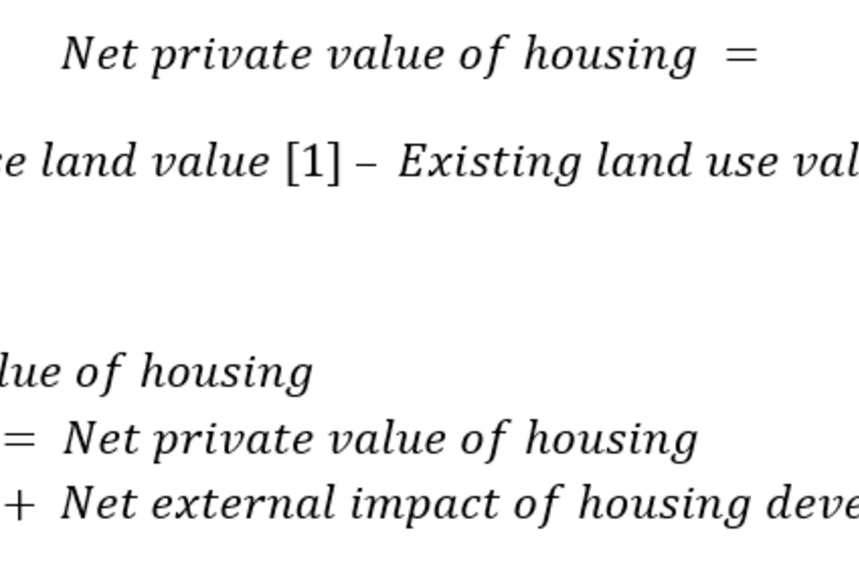
B6. A range of infrastructure is required to facilitate new development, including water, sewerage and electricity connections. The impacts of granting planning permission may be attributed jointly to the land use development and any accompanying infrastructure improvements, including those relating to transport. It would not be appropriate to ascribe the impacts to the development in isolation.

B7. Note that costs of infrastructure, whether borne by developers or by the exchequer, do not affect the overall valuation of the change in land use outlined above. However, the incidence of infrastructure costs does have distributional effects – to the extent that developers contribute towards these costs, we would expect the costs to be ‘passed back’ to landowners in the negotiated price of undeveloped land, so reducing the surplus that otherwise accrues to landowners on the grant of permission.

Residential land value [1]

B8. The residual method of land valuation gives the maximum price a firm is willing to pay for land for development. As noted in Chapter 4, the developer will also incur costs and would expect a minimum level of profit from developing a site. In a competitive market, the firm will pay a price that gives a normal level of profit.

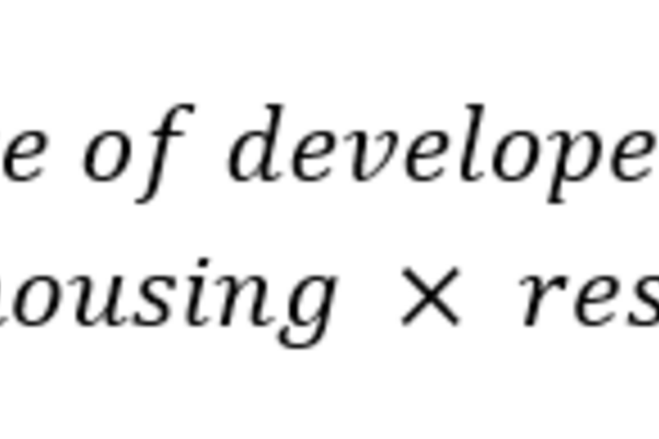
B9. Users must firstly calculate the hectarage of housing. The total value of the land in planned residential use is then estimated by multiplying that hectarage by a per hectare residential land value. Alternatively, the residential land value may be estimated by other means, for example:

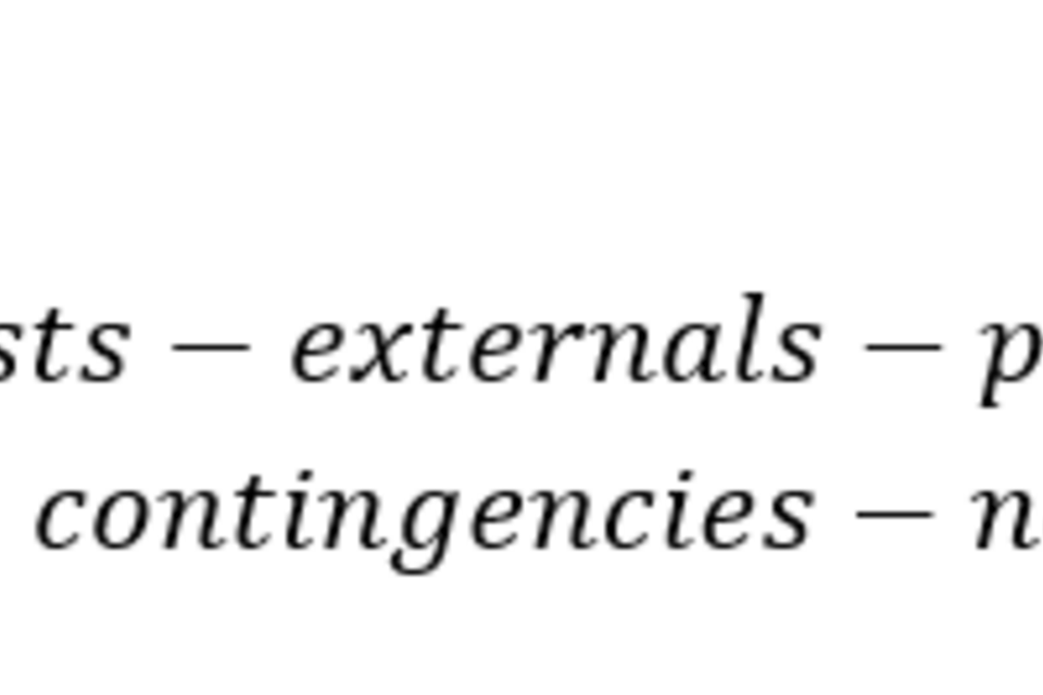
B10. Any abnormal costs not covered in the above values should then be netted off as a disbenefit to the private sector.

B11. For appraisal, the Green Book advises that ‘Transfers of resources between people (e.g. gifts, taxes, grants, subsidies or social security payments) should be excluded from the overall estimate of Net Present Social Value (NPSV).’ Market land values are reduced by affordable housing requirements, which allocates a proportion of the total value to society of new housing towards building additional affordable housing.

B12. The values published in DLUHC ‘Land value estimates for policy appraisal’ are already adjusted in this way, so as to provide values for appraisal which reflect the full value to society of new housing. Where local land value estimates are used these should also be prepared so as to exclude, for example, the impact of affordable housing requirements on prices.

Existing land use value [2]

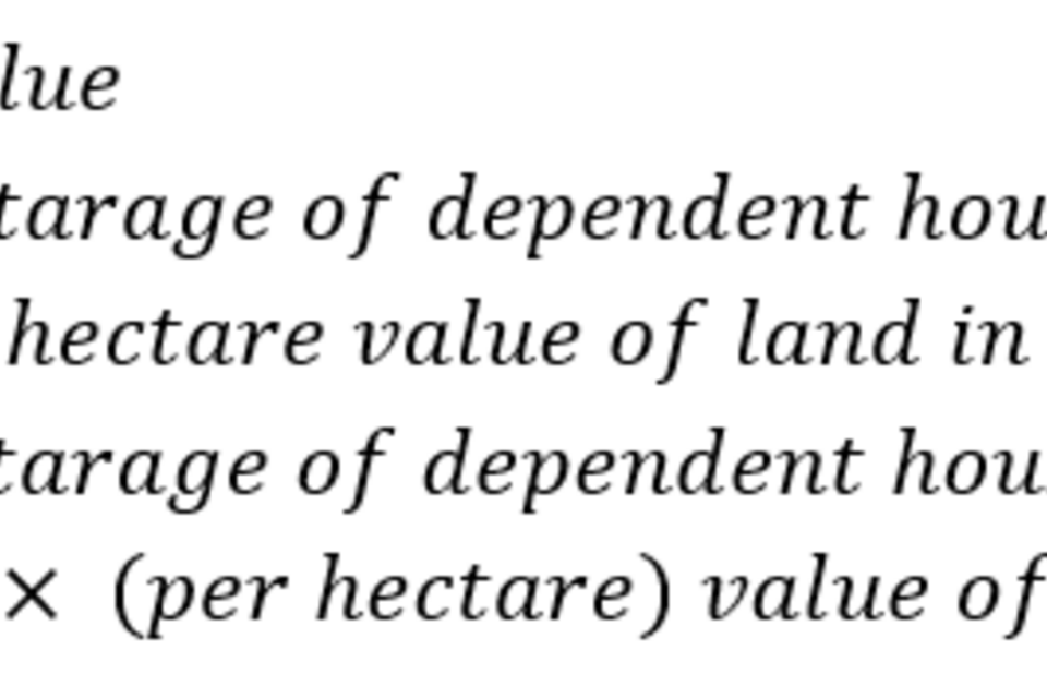
Note: PDL = previously developed land

B13. Users must then calculate the hectarage split between previously developed land (PDL, also known as ‘brownfield’) and undeveloped land (non-PDL, also known as ‘greenfield’), of the land for residential development. The overall value of the land in existing use is then estimated by multiplying the PDL and non-PDL hectarages by corresponding per hectare values.

B14. For PDL, a regional-level per hectare value for industrial and warehouse land can be used; for non-PDL, a regional-level per hectare value for agricultural land in mixed use can be used. The DLUHC Land value estimates for policy appraisal contains average value estimates for industrial and agricultural land in England, though users may draw upon alternative sources of evidence to inform estimation of land values in areas of dependent development.

Net external impact of housing development [3]

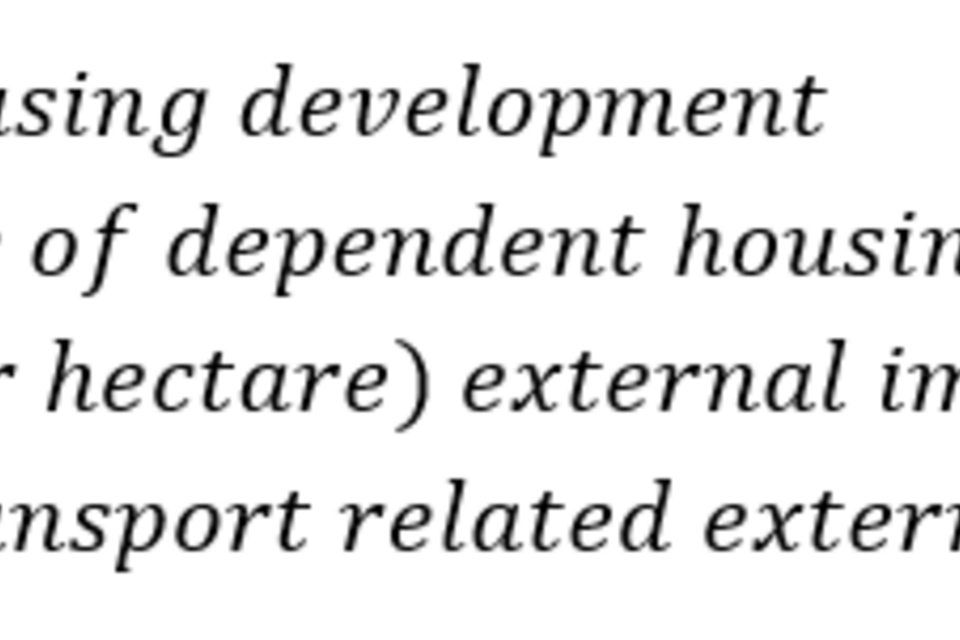
B15. The existing hectarage split between PDL and non-PDL for development is also used to estimate the overall value of the external impact of the development. For non-PDL, estimates of the external benefits of undeveloped land are set out in Annex G. The mean average of the reported estimates of external benefits of 4 types of land: urban fringe (forested land), urban fringe (greenbelt), intensive agricultural land and extensive agricultural land can be used.

B16. For PDL, the external impact of development has not been monetised, though in certain circumstances redevelopment might bring external benefits through, for example, improving the aesthetic value of the area surrounding the development (see Annex G).

B17. Users may draw upon alternative sources of evidence to inform estimation of the external impacts of development.

B18. As noted earlier, there is a further external impact of development to be considered in the overall valuation - the transport costs imposed on existing users of the network by residents of the new development. These transport-related external impacts of development should be added to the non-transport-related external impacts discussed above (see Annex G for further details).

Qualification to [3] when applying the wider area impacts approach

B19. In regeneration areas, to avoid double counting, the wider area impacts approach set out in Annex G should be used rather than the external impacts identified in equation [3]. Annex G provides a calculator to assess impacts in regeneration areas.

Development in future years

B20. For any additional housing that is expected to be delivered in future years, land value uplift should be uprated in line with real GDP growth each year. This assumption is in line with the discussion set out in the house price and land value growth sections. To simplify and in the absence of further data, we assume that this applies to all elements of net social land value uplift including agricultural land values, industrial land values, and externality values.

B21. Given the uncertainty surrounding future house prices it is recommended that sensitivity analysis is carried out to test the robustness of the results. The sensitivities to be applied will depend on forecast GDP growth, but a reasonable range would be:

A low sensitivity given by nominal growth in line with price inflation (that is a 0% real increase in house prices and LVU per annum); and
A high sensitivity of a 5% increase in house prices and land value uplift above inflation, which is consistent with previous appraisal guidance assumptions.

Question 13

Annex C: Land value uplift for non-residential development

Accepted Answer

C1. This Annex describes DLUHC’s approach to valuing the impacts of non-residential development.

The preferred approach involves the use of local land value data to assess the private costs and benefits of a policy.
In the absence of reliable local land value data, an approach using illustrative VOA land value data is outlined.

C2. Even where local data is available it may be useful to cross-check estimates using VOA data. Large discrepancies should be investigated further to find out what is driving them.

The approach

C3. The value to society of a planning decision to grant permission for new non-residential development may be separated into:

The private benefit associated with the change in land use, as represented by the uplift in value arising from the land moving from its current use to a more productive use. This uplift is defined as the value of the land in its new use (in this case commercial) minus the value of the land in its existing use (e.g. agriculture); and
The net external impact of the resulting development, including any loss or gain in amenity.

C4. The equation below summarises this:

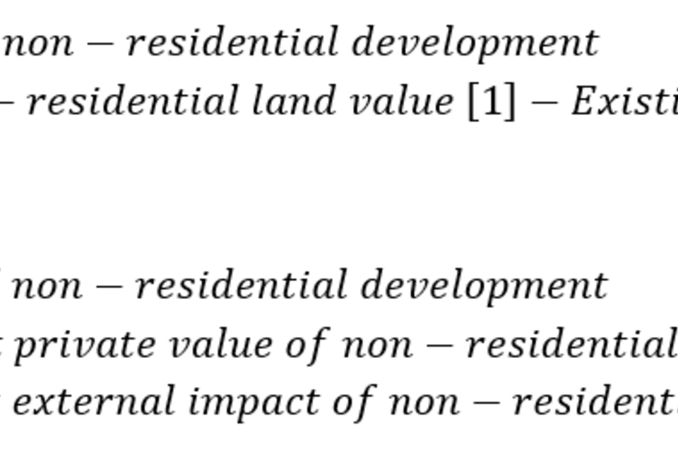
The calculation

C5. Below is a discussion of the key elements of the appraisal, including the data inputs and underlying assumptions. Note that a number of data inputs must be specified by the user on a case-by-case basis as they relate to the nature of the development in question.

Non-residential land value [1]

C6. The total value of the land in planned non-residential use is estimated by multiplying the hectarage of land by a per hectare non-residential land value.

a) Locally available land value data is available

C7. Where possible locally derived land value data should be used to estimate the land value from post-development. It should be noted that in practice land values vary substantially on a site-by-site basis, given differences in, for example, proximity to amenities or density of development. As land value estimates are one component of subjective residual valuations made by developers, it is important that an explanation for how these estimates are derived is clearly set out in the economic dimension of a business case:

C8. Users are encouraged to draw upon alternative sources of evidence to inform estimation of land values in areas of dependent development. Any site values based on recent sales should be consistent with the intended development on:

Business use of site: for example commercial property can be used as an industrial plant, a logistics warehouse, a hi-tech lab or as office space and the value generated by each of these developments is very different.
State of development of site: represent typical levels of value for sites that are ripe for development, in that they have the following conditions:
- no abnormal site constraints;
- a planning permission of a type generally found in the area; and
- services to the edge of the site.
Measurements: the size of the site should be consistent.

b) Locally available land value data is not available

C9. The preference is to use locally derived land value data to estimate both the existing land value and future non-residential land value. Where these are not available, typical values estimated by the VOA can be used.

C10. The VOA provides non-residential land value estimates at Local Enterprise Partnership (LEP) area level. Values are available for agricultural use, industrial use and commercial use. For industrial and commercial values, estimates for multiple areas within LEP area are available and users should use their judgement as to which is most appropriate for the area they are appraising. For commercial values, values are available for both city centre and out of town offices (or for London, inner or outer London) and again users should use their judgement as to which is appropriate. VOA’s non-residential land values should be regarded as illustrative and represent typical levels of value for sites for development. They should be regarded as being at market prices (that is gross of indirect tax).

C11. As noted above land values vary substantially on a site-by-site basis, given differences in, for example, proximity to amenities or density of development. Users are therefore encouraged to draw upon alternative sources of evidence to inform estimates of land values.

C12. The economic dimension of the business case should clearly set out the justification for choices made in use of land value data.

Existing land use value [2]

C13. Where locally available data is available users may draw upon those sources of evidence to inform estimation of land values.

C14. Where locally available data is not available then typical values estimated by the VOA can be used.

Net external impact of housing development [3]

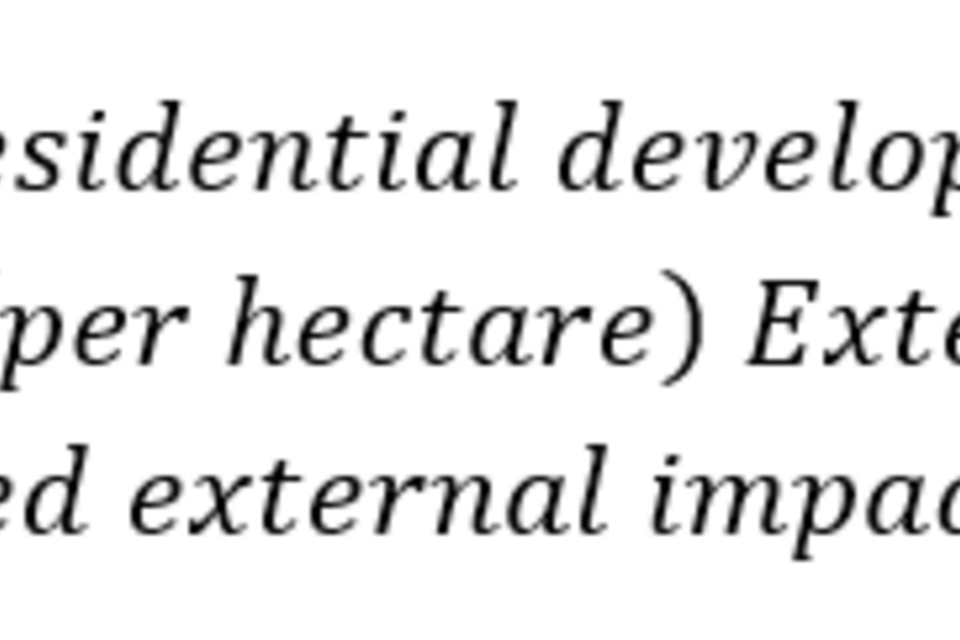
C15. Users may draw upon alternative sources of evidence to inform estimation of external impacts of development. A conservative assumption may be to assume that the net external impact of non-residential development is zero even though redevelopment may bring external benefits through, for example, improved aesthetic value of the area surrounding the development.

C16. The overall benefits related to the development are therefore:

In which the land value uplift estimate captures the net private benefits and the net external impact captures externalities such as changes in amenity.

Costs

C17. All public sector costs should be included. If the land is owned by the public sector then it will be incurring holding costs. These costs include, for example, maintenance of land and buildings on the site, maintaining its security and environmental standards. In the absence of site specific evidence these can be assumed to be 2% of the existing value of the land per year (see holding costs). Should the land be developed then these holding costs will be avoided. This needs to be reflected in the appraisal as a negative cost. Any private costs associated with the development should be included in the appraisal as a disbenefit and therefore feature in the numerator of the BCR calculation.

Appraisal period

C18. Expected to be 10, 30 or 60 years, depending on the intervention being appraised.

Timing

C19. The land value uplift is assumed to happen at the same time as a change in land use. There is no assumption that benefits are built slowly over a specified time period. All other costs and benefits will need to be discounted at 3.5 per cent per annum in line with the HMT Green Book.

Multiple sites

C20. Where there are multiple sites an overall BCR may be calculated provided there is a positive uplift on all sites.

Additionality

C21. Not all economic activity associated with the land value uplift of an intervention will be additional – some will be displaced from other locations and some might have occurred in the absence of the intervention (deadweight). As a result, in an economic appraisal the land value uplift associated with an intervention should be adjusted for additionality.

C22. For example, it would be expected that the additionality of the land value created would be relatively high for an intervention where there is strong market failure (e.g. access to finance), a strong strategic rationale (e.g. clustering of similar industries meaning investment in an alternative location is unlikely), where the development is in a low displacement sector and where there is limited alternative uses for the land. Where these considerations do not hold additionality is likely to be significantly lower. Annex D provides some illustrative values to use when assessing additionality.

A worked example

C23. Assume a policy option being appraised is a grant of £3.7m for the second phase of works at a 39 acre site owned by the public sector. The land is highly contaminated and the grant is to be used to remediate the land. The remediation of the land would enable businesses to move to an area where there is an existing cluster of businesses in a highly productive sector. Also assume that an additional £4.2m of infrastructure works including road and electricity works simultaneously goes ahead to increase the site’s commercial viability. These costs were incurred by the public sector. The land is publicly owned with holding costs of approximately £65,000 per year.

C24. There is data available on the current value of the land and the value of the land post remediation. The future land value estimate is based on the sale of a piece of land in a similar state of development and to be used for the same business use.

Table 8: Worked example for non-residential development

Factor	Detail
Site area	39 acre ( ≈ 15 hectares)
Primary cost	£3.7m grant for remediation
Other costs	£4.2m infrastructure works in the first year. A negative holding cost to the public sector without intervention (assumed £65k per year)
Existing use land value estimate	£30,659 per acre
Future use land value estimate	£200,000 per acre

C25. Costs: the costs are valued as the net present value costs to the public sector. The costs include the £4.2m infrastructure works and the £3.7m grant less the negative (avoided) annual public holding cost of £65k. Using the 3.5% discount rate this gives a net present public sector cost of £7.1m (appraised over 10 years for simplicity).

C26. Net private value: the net private value is calculated using the land value estimates set out above. The new use land value of £200k per acre gives a total value of £7.8 million over 39 acres.^{[footnote 44]} Subtracting the £1.2 million^{[footnote 45]} existing land value (before remediation) gives a net present private value of £6.4m rounded to the nearest hundred thousand and after discounting by 3.5 per cent to reflect the fact it takes a year to remediate the land.^{[footnote 46]}

C27. Net external impact: the net external impact is estimated to be zero. This is a conservative estimate since there may be an amenity value from the redevelopment. Therefore, the present value benefit of the development is £6.4m.

C28. ‘Initial’ and ‘adjusted’ BCR: the ‘initial’ and ‘adjusted’ BCR before an additionality factor is applied is:

C29. Additionality: the above calculation assumes 100% additionality, that is that the firm which ‘takes over’ the site only does so as a result of the intervention and there is no displacement of economic activity elsewhere. However, although it is reasonable to argue that there would be no deadweight (given the BCR is less than one indicating such an investment by the private sector would not happen as it would not be commercially viable), there may still be some displacement of economic activity from elsewhere.

C30. Sensitivity analysis: sensitivity analysis can be used to see how the BCR might change if assumptions were altered with respect to additionality. Sensitivity analysis should look at both costs and benefits. For example:

a. Benefits – it might be that the land price after intervention is overly optimistic or only a proportion of the site is wanted by firms so that benefits are lower. If this occurred and benefits were reduced by for example 10%, the BCR would fall to £5.8m/£7.1m = 0.8.

b. Costs – Alternatively the costs of remediation or of additional public sector infrastructure might be different from central estimates. Three illustrative examples are shown in the table of a 40%, 100% and 150% increase in total costs (initial land value, remediation + other infrastructure-less holding costs).

C31. For example, a 100% increase in costs leads to BCR=£6.4m/£14.2m = 0.45. The BCRs for the other two cost increases are shown in the table below.

Table 9: BCRs with varying levels of optimism bias

	10% lower benefits	40% higher costs	100% higher costs	150% higher costs
BCR	0.80	0.65	0.45	0.35

C32. Switching values: sensitivity analysis can also be used to identify a ‘switching value’ where the VfM moves to a different band. This can be used to examine non-monetised impacts as well as uncertainty in monetised impacts. In the example the potential for amenity benefit from the development is examined. The question is, “How big does this amenity benefit need to be for the BCR to be 1, 1.5 or 2, for example?”

Table 10: Increase in land values required from external amenity impact to shift to new BCR

	BCR = 1	BCR = 1.5	BCR = 2
Required additional benefits for given present value costs of £7.1m	£700,000	£4,250,000	£7,800,000
Additional amenity value required per acre (to nearest £1000)	£18,000	£109,000	£200,000

C33. As the sensitivity analysis shows, the BCR of the development could fall to as low as 0.65 if Optimism Bias of 40% was applied to the costs of the remediation. The BCR could be 1 if the post-remediation value of the land was approximately £18,000 per acre higher than the £200,000 it has been estimated at, or if the value of the net external impact of development was valued positively at 11% of the value of the private benefit instead of being valued at zero. With no other impacts to consider – and given that the size of the amenity benefits needs to be relatively large even if 100% additionality is assumed – then this policy option could be considered Poor value for money.

Question 14

Annex D: Estimating additionality

Accepted Answer

D1. This chapter provides guidance on quantifying the size of the additionality for residential and non-residential developments.

D2. Additionality is the real increase in social value that would not have occurred in the absence of the intervention being appraised. For developments the key factors involved in assessing additionality are:

a) Deadweight – defined as the level of target outputs/outcomes that would have been produced if the intervention did not go ahead. This involves estimation of what scale and type of development, if any, would have taken place on the site in the absence of intervention, and over what time frame.

b) Displacement – defined as the level of outputs/outcomes (occurring under the counterfactual and the intervention options) accounted for by reduced outputs/outcomes elsewhere in the target area.^{[footnote 47]}

D3. Where interventions are targeted on particular areas (e.g. through levelling up) or target groups (e.g. low income groups or particular industries/commercial groups) then leakage also becomes relevant. This represents the proportion of outputs that do not go to the target group/area. High rates of leakage indicate that that the intervention is failing to achieve its key objectives. Analysis of leakage is a key part of distributional analysis.^{[footnote 48]}

D4. To estimate the correct level of additionality it is essential to properly determine the counterfactual and work through the logic model of the intervention. This involves clarifying the chain of causation through which inputs translate into outputs and outcomes, both desirable and otherwise.

D5. The approaches to measuring additionality in residential and non-residential developments are set out below.

Box 4: The link between additionality and VfM

There is a direct link between the size of the additionality associated with a policy option and the estimated VfM. This is particularly important to note when private benefits represent a significant proportion of overall benefits. When this is the case, in the absence of a sound rationale for intervention such as a market failure, it would be reasonable to assume that in the absence of government intervention these private benefits would materialise anyway.

This would suggest such a policy option would have significant deadweight and minimal additionality, and therefore be poor VfM. However, where there is evidence of a market failure preventing a development from taking place in the absence of government intervention, it would be reasonable to assume there is less risk of deadweight and greater levels of additionality associated with the policy (meaning higher VfM).

Additionality for residential developments

D6. Three key factors determine the extent of additionality.

The degree to which there is a clear market failure which means that market outcomes are suboptimal (e.g. development is too low because of failure to take account of positive externalities, or there are credit constraints on small builders due to asymmetric information);
Whether the focus of the intervention is on the demand or supply side of the residential market. Demand side policies tend to have higher elements of displacement than supply side policies as they do not initially increase the volume of housing stock (that occurs in response to subsequent price increases)^{[footnote 49]}; and
The point in the housing cycle. In economic upswings housing interventions are likely to be in greater competition for resources with existing planned activity, leading to greater displacement.

D7. Ex-ante assessment of additionality is often extremely difficult to quantify, and therefore any figures used should be subject to rigorous sensitivity analysis as part of the appraisal. Users may wish to calculate a switching value of additionality that gives an overall BCR of 1 (or NPSV of zero) for the policy, that is, what number or percentage of dwellings would need to be genuinely additional in order for benefits to exactly equal costs.

D8. The following bullets set out potential additionality assumptions that could be used in the absence of alternative evidence to help inform the value for money of a housing intervention:

0-25% additionality: policies which fall into this category will be demand focussed. The market failure underpinning the intervention may also be less prevalent than in the past (such as access to finance, though we may still expect this to be significant for Small and Medium Enterprises). These policies are therefore likely to have a very large amount of deadweight and displacement associated with them.
25-50% additionality: policies which fall into this category may be demand or supply focussed but the level of additionality is higher because of the point in the housing cycle when the intervention takes places, and / or because the market failure (ideally supported by local evaluation evidence) is stronger. For example, the policy may be targeted at a particular group like Small and Medium Enterprises (SMEs) or first time buyers. Deadweight or displacement is likely to be large.
50-75% additionality: policies which fall into this category will usually be supply focussed with good supporting evidence justifying the additionality assumption. Deadweight and displacement are likely to be relatively small. An example would be Affordable Housing where there is strong evidence to suggest housing of this type is unlikely to be built by private developers in the absence of policy and very little crowding out of private development occurs in practice.
75%+ additionality: policies which fall into this category will usually have a strong supply focus with good supporting evidence. Deadweight and displacement are likely to be small. For example, it could cover a situation where there are relatively high ‘clean-up’ costs which mean the site is unviable (and so would not go ahead in the counterfactual) and there are no other sites available in the local area. There could also be a condition of funding that housing would need to be delivered on top of local plans. The site may also be located in an area of high housing need. General economic conditions might also be relatively muted, maximising any additional impacts on the demand side (if applicable).

Specific evidence for supply side housing interventions

D9. Specific evidence on the additionality of supply side housing interventions has been developed by Amion. Amion has calculated deadweight and displacement ready reckoners to provide approximate estimates of each impact. Figures 4a and 4b below show the ready reckoner flowchart for both deadweight and displacement. These should be followed to calculate deadweight and displacement for supply side housing interventions.

Deadweight ready reckoner

D10. In most cases the preferred approach to assessing deadweight is to construct a bespoke counterfactual built on evidence-based judgments. However, as a general guide to analysts, a deadweight ready reckoner is provided to indicate how the deadweight associated with supply-side housing projects could be assessed.^{[footnote 50]} It provides a plausible range of deadweight values associated with different types of project. The degree of deadweight that should be applied will vary according to judgement of the significance of individual factors and the strength of the evidence.

Displacement ready reckoner

D11. The displacement ready reckoner is based on regression analysis carried out by Amion to estimate displacement associated with government supported projects. It is designed to be used to support the estimate of displacement for supply-side housing projects. Key factors affecting displacement have been identified as local housing market affordability; development activity in the local area; the scale of the development; and the proportion of homes that are non-market homes.

D12. To estimate total additionality the following formula should then be used once the deadweight and displacement calculations have been made:

Additionality = (1 - deadweight) * (1 - displacement).

D13. There are two important caveats to these ready reckoners:

They should only be applied to supply side housing interventions.
They do not assess leakage, place based or distributional impacts. Where these are judged to be important by the user, further analysis would need to be done to understand their impacts in line with the Green Book Annex A2 and A3.

Figure 4a: Flowchart for calculating deadweight

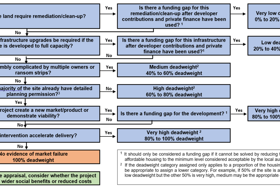
Figure 4b: Flowchart for calculating displacement

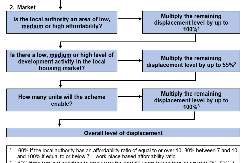
Box 5: Example of the application of deadweight and displacement calculators

A local authority is bidding for £1m to unlock a site which will release 1.5 ha of brownfield land for the residential development. The final site will have 60 units, of which 20 units will be affordable or social rent. It is currently a riverside industrial site with significant decontamination costs, demolition, and flood defence requirements, for which the local authority is seeking a grant to part meet costs. The bid includes an industry standard valuation of the site and an estimate of the cost of works based on similar schemes. The affordability ratio in the local authority is 8.5, and the total net additions to stock over the past 10 years is 6.5%.

Deadweight – The deadweight of the scheme is assessed as between 0% and 20%, with a central estimate of 20% to reflect that a proportion of the site is likely to be developed in the future without addressing the abnormal costs in the remainder of the site. Most of the land within the site requires significant remediation and clean up before it can be used for development. There is clear evidence from the site-specific valuation that it is the additional costs related to this that creates a funding gap / viability issue which will prevent most of the site being developed. There are no reasonable changes to the scheme, such as reducing the proportion of affordable housing, that would be acceptable within local planning guidelines.

Displacement – the level of displacement depends on the proportion of social/affordable rented housing, the level of affordability, the level of development and the number of units built. Based on the example:

Displacement = (1 – proportion of social/affordable rent) x medium affordability (80%) x medium development activity (50%) x number of units (40%)

= (1 - 0.33) x 0.8 x 0.5 x 0.4 = 11%.

The final additionality of the scheme is (1 – deadweight) x (1 – displacement)

= (1 – 0.2) x (1 – 0.11) = 71%.

Additionality for non-residential developments

D14. As Chapter 4 explains, one way of accounting for potential displacement and deadweight is to adjust the gross land value uplift estimates of an intervention. To guide users on how this adjustment could be done, the framework set out in Figure 5 could be used in conjunction with sensitivity analysis in a non-residential appraisal. Please note, the sizes of the adjustment factors are purely a guide. If there is evidence on the appropriate size of these adjustment factors then this should be used in the first instance. In the absence of this information, the illustrative figures can be used.

D15. The framework in Figure 5 sets out various criteria that would need to apply for there to be minimal displacement and deadweight from a particular intervention. For example, the existence of a market failure and strong strategic rationale for a development coupled with the industry under consideration being in a relatively low displacement sector would lead to high additionality being assumed. This might be a firm wishing to expand in a geographic area where there is a clustering of industry it would benefit from being near to but being unable to do so because of a failure in the lending market. In this case a relatively small downward adjustment would be made to the gross land value, for example 75% of the gross land value might be used in the appraisal.

D16. On the other extreme, where there is a weak market failure and strategic rationale for intervening, and where the industry under consideration suffers from significant displacement (such as retail), the gross land value would be significantly adjusted downwards, with the net impact being 25% or less of the gross land value created.

D17. The levels of existing vacancy rates in the non-residential sector will also be important. Where vacancy rates are high for the relevant sector then levels of additionality are likely to be low and additionality assumptions should be adjusted to reflect this.

D18. Analysts will need to exercise judgement on the appropriate size of the adjustment to use taking into account the criteria below. As part of any sensitivity analysis, it may be useful to calculate a ‘switching value’ that is the size of the additionality factor required to make the development NPSV positive.

D19. The sensitivity analysis on the land value estimate, as well as the potential for non-monetised impacts and the externalities in Annex G, should inform the value for money category and ‘adjusted’ BCR. In particular, this sensitivity analysis will be useful in arriving at an overall judgement on the value for money category and the range it takes.

Figure 5: Additionality framework for non-residential development

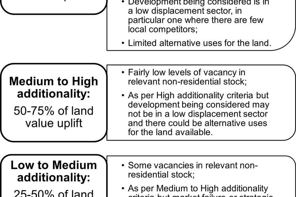
High additionality: 75-100% of land value uplift

No or very low levels of vacancies in relevant non-residential stock;
Strong market failure e.g. market failure in the lending market;
Strong strategic rationale e.g. development is part of a clustering of industries which benefit from being together, meaning investment in an alternative location is unlikely;
Development being considered is in a low displacement sector, in particular one where there are few local competitors;
Limited alternative uses for the land.

Medium to High additionality: 50-75% of land value uplift

Fairly low levels of vacancy in relevant non-residential stock;
As per High additionality criteria but development being considered may not be in a low displacement sector and there could be alternative uses for the land available.

Low to Medium additionality: 25-50% of land value uplift

Some vacancies in relevant non-residential stock;
As per Medium to High additionality criteria but market failure or strategic considerations are less strong.

Low additionality: 0-25% of land value uplift

High/very high vacancies in relevant non-residential stock;
As per Low to Medium additionality criteria but development being considered is in a high displacement sector such as retail.

Question 15

Annex E: Homes England residential optimism bias calculator

Accepted Answer

Optimism bias on capital costs

E1. This Annex provides advice to support analysts in applying the HMT Optimism Bias (OB) supplementary guidance so that it is applied consistently.

E2. There are two parts to this annex:

The first provides support in defining the categories of spend used within the supplementary OB guidance; and
The second considers the contributory factors to the upper bound rates discussed within the supplementary guidance and how these might be mitigated.

Spend categories

E3. The table below provides the upper and lower bounds presented in the Green Book supplementary guidance on OB. The upper bound reflects the average OB found for traditionally procured projects pre-procurement and the lower bound reflects the level of OB to be applied at the point of contract award for projects with effective risk management. The starting point for projects will be the upper bound.

E4. For larger projects it may be necessary to undertake an assessment of OB separately for each phase in recognition of the different stage of development of those phases. For example, if there was an early phase that was already contractually committed the lower bound OB may be appropriate, whereas for a future phase yet to be developed the upper bound might be applied.

Category	Capital Expenditure Optimism Bias % - Upper	Capital Expenditure Optimism Bias % - Lower
Standard Buildings	24	2
Non-Standard Buildings	51	4
Standard Civil Engineering	44	3
Non-Standard Civil Engineering	66	6
Equipment/Development	200	10
Outsourcing	41	0

E5. Within the Green Book supplementary guidance and other associated documents, several definitions are provided to help to explain the categories of spend included in the table above. The table below aligns these categories with definitions applicable to residential and commercial development projects.

E6. When considering these definitions, it may be necessary to divide a project into several component parts so that the relevant level of OB can be applied to each component. For example, where a project involves constructing a new school building and a new road there may be elements of buildings and elements of civil engineering.

E7. The breakdown by these components can then be used to generate a blended OB rate that can be used as an input to the appraisal model.

Category	Definition
Standard Buildings	The construction of buildings where a standard approach to design can be used. For example, where there is a greenfield site with few constraints impacting on design. Buildings could include the construction of offices, living accommodation or schools.
Non-Standard Buildings	The construction of buildings where a non-standard approach to design is required. Characteristics of a site where a non-standard approach is required may include; • Space constraints • Brownfield sites • Refurbishment projects • Innovative buildings • Other complicated site characteristics Buildings could include the construction of offices, living accommodation or schools.
Standard Civil Engineering	Those facilities, in addition to buildings, where no special design considerations are required. For example, where there is a greenfield site with few constraints impacting on the design. Facilities could include the construction of roads and utilities.
Non-Standard Civil Engineering	Characteristics of a site where a non-standard approach is required may include; • Space constraints • Brownfield sites • Other complicated site characteristics • Unusual output specifications • Innovative transport infrastructure or upgrade/extension projects • Innovative utility projects Facilities could include the construction of roads and utilities.
Equipment/Development	The provision of equipment and/or the development of software and systems.
Outsourcing	The provision of hard and soft facilities management services.

Contributory factors and mitigations

E8. Within the Green Book supplementary guidance percentage contributions to the upper bound rates are given for a series of contributory factors, allowing for the upper bound OB rate to be reduced based on an assessment of the extent to which each has been mitigated within the scheme.

E9. To standardise the process for the assessment of development schemes, we pose a series of questions linked to these contributory factors. The responses to these questions will then be used to apply a standardised set of mitigation factors to the upper bound OB rate.

E10. Consideration should be given to whether the responses to the questions would be the same for all options under consideration or whether the responses and so level of OB may need to vary by option.

E11. The table below lists these questions, the responses and proposed level of mitigation of the associated contributory factor by response. These are based on the detail within the appendix to the Green Book supplementary guidance and Appendix E from the 2002 Mott MacDonald study.

E12. Those listed as N/A relate to categories not linked to capital cost mitigations for buildings or civils within the Greenbook supplementary guidance. We also assume no mitigation against the ‘other’ categories listed.

Question 16

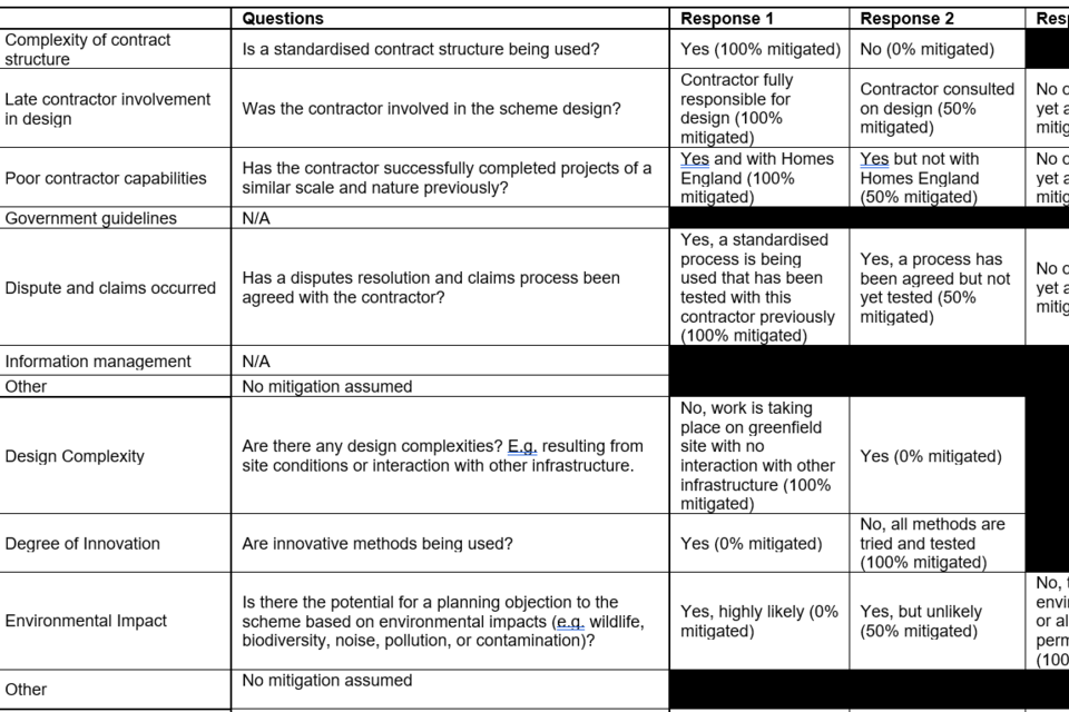
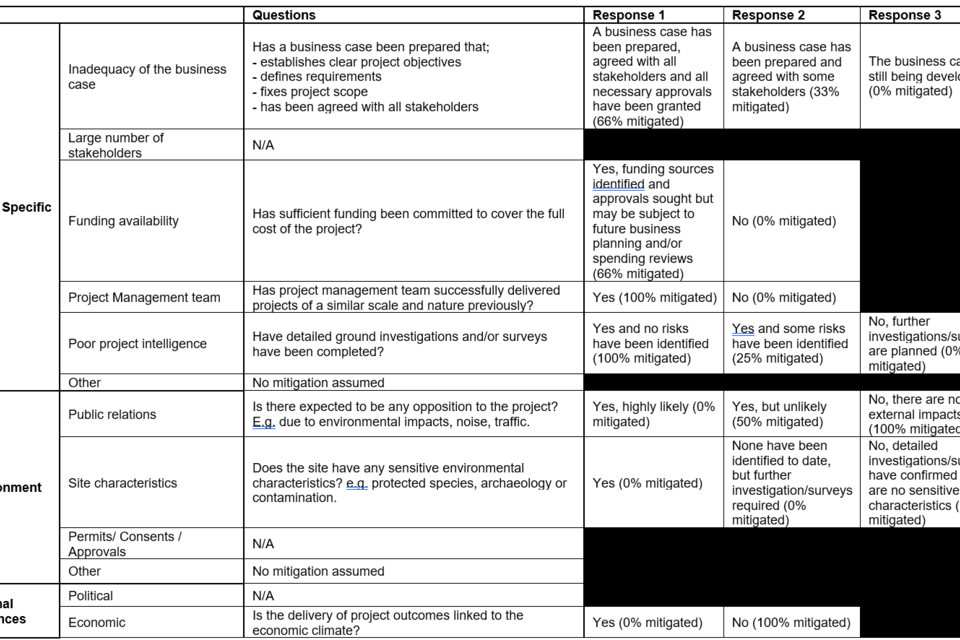
Annex F: Market failures

Accepted Answer

F1. Public sector intervention can be based on strategic objectives, improvements to existing policy, market failure or distributional objectives that the government wishes to meet. Market failure is one rationale for intervention and exists when the market mechanism alone cannot achieve economic efficiency in the allocation of a good or service.

F2. In welfare economics, an inefficient outcome means social welfare can be increased without making other parties worse off – that is, by correcting market failure, social value will increase. This definition does not mean that it is appropriate for the public sector to deliver whatever the market will not. There needs to be sufficient social value in doing so and not unduly displacing market activity.

F3. The table below outlines instances of market failure which are particularly relevant in a DLUHC context but is not exhaustive.

Table 11: Sources of market failure

Type of Failure	Definition
Public good	A public good can be defined by two characteristics: firstly, it is difficult to exclude anyone from enjoying it (non-excludable in supply); and secondly, once provided, a person’s consumption of the good does not stop anyone else from consuming it (non-rival in demand). A public good will be both non-rival and non-excludable.
Externalities	Externalities arise when an activity results in benefits or costs to people other than those directly producing or consuming the good. A failure to properly consider these external impacts will result in socially sub-optimal outcomes. A common example of a negative externality is pollution, where those causing the pollution do not bear the full costs. In contrast, an intervention to redevelop a derelict site to provide new housing is an example of a positive externality through the impact it can have on improving the amenity of the surrounding area.
Coordination failure	Coordination failure refers to when a socially desirable activity does not take place due to a failure to coordinate effectively between the different parties involved. For example, a development scheme may require agreement between multiple land owners but this is not possible in the absence of public sector intervention due to competing or incompatible objectives.
Market power	Market power results from insufficient competition to ensure a market operates efficiently. Sectors such as housebuilding have high barriers to entry and existing businesses may act strategically, through predatory pricing, taking options on land or land banking, to deter competition.
Imperfect information	Imperfect information happens when buyers and sellers do not have all the information they need to make a fully informed decision. Buyers need to know the quality of a good or service to judge the value it can provide. Sellers, lenders and investors need to know the reliability of a buyer, borrower or investor. If information is asymmetrical, this can lead to adverse selection and the market may not operate efficiently.

Approach to assessing market failure

F4. When building a case for market failure it is helpful to consider the following points:

Proportionality should always underpin market failure assessment. Large, novel or contentious projects will inevitably require more detailed work.
When considering market failure arguments and reviewing evidence, thought should be given to how potential causes of market failure may evolve over time.
It is important to understand all the reasons the market alone will not deliver efficient outcomes for society (for example, there might be more than one factor which needs to be addressed through public sector intervention). Taking this holistic view will be crucial in helping decide if and how a scheme should come forward using public sector intervention.

Question 17

Annex G: Externalities associated with development

Accepted Answer

Background

G1. An economic appraisal should seek to capture all the benefits and costs of an intervention. This includes private benefits – such as land value uplift – and external impacts which often represent an important element of overall impacts. Where possible these impacts should be monetised.

G2. There are a number of external impacts that are likely to result from a development including placemaking and regeneration impacts, potential agglomeration impacts on third parties, health impacts of additional affordable housing and brownfield land clean-up, educational impacts of additional housing, transport externalities, environmental impacts, and cultural and amenity impacts of development (see Figure 6 below).

G3. Users should draw on appropriate evidence and guidance to take account of and value these impacts. For DLUHC appraisals, to ensure consistency and transparency on what is included in an economic appraisal, only impacts that can be robustly valued using (Supplementary and Departmental) Green Book guidance should be included in the estimate of an ‘initial’ BCR. Examples of such impacts include safety impacts, congestion impacts, air quality and greenhouse gas emissions. Amenity impacts, placemaking and distributional impacts should be monetised separately and included in an ‘adjusted’ BCR. Distributional impacts are discussed in Annex H.

Determining whether an impact is an externality

G4. When assessing externalities, it is important to consider whether an impact is already captured in land value uplift. If it is not then it is an additional impact that needs assessing. The framework below in Figure 6 sets out an approach to doing this.

G5. The key question to ask of a potential impact is, “Who does it affect?”

If the impact affects the welfare of an individual or firm moving to an area, then this impact may be fully reflected in the price they pay for the thing they are buying, for example a home. Where this is the case, these impacts should not be considered an externality.
If the impact affects the welfare of individuals or firms already in the area, then this impact will not be accounted for in land value uplift and is therefore an externality.
If the impact affects society as a whole (so not exclusively existing individuals or firms in an area), then this impact will not be accounted for in land value uplift and is therefore an externality.

G6. Thus when locating to an area a firm will consider whether there are any potential spill-over benefits to it from co-location with other firms (agglomeration impacts) and the costs to the firm from local road congestion. This will affect the price it is prepared to pay for a development. Individuals moving to an area will also factor the characteristics of the external local environment such as any congestion or amenity benefits when they are deciding how much to offer for a property and this will also be factored into land value uplift.

G7. However, land value uplift will not account for impacts which affect existing firms or individuals in an area (or society as a whole). These are externalities. For example, any knowledge spill-over impacts enjoyed by existing firms from a new development will not be taken into account by the firm deciding to locate in an area so are in addition to land value uplift. Similarly, the firm or individual deciding to locate in an area will not take into account the congestion cost they impose on others. These impacts are externalities which need to be accounted for in addition to land value uplift.

Examples of valuation of externalities

G8. To help guide users, this annex provides illustrative examples of the calculation of three types of externality:

Gi Assessment of wider placemaking impacts in regeneration areas;
Gii The health impacts of affordable housing;
Giii Amenity impacts resulting from changes in land use.

Figure 6: Framework for assessing externalities

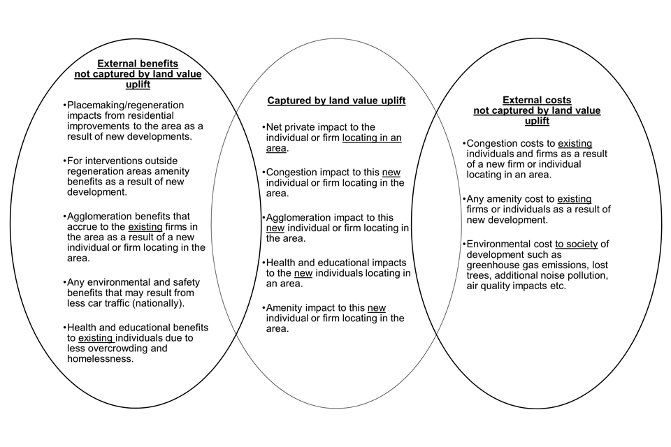
External benefits not captured by land value uplift

Placemaking/regeneration impacts from residential improvements to the area as a result of new developments.
For interventions outside regeneration areas amenity benefits as a result of new development.
Agglomeration benefits that accrue to the existing firms in the area as a result of a new individual or firm locating in the area.
Any environmental and safety benefits that may result from less car traffic (nationally).
Health and educational benefits to existing individuals due to less overcrowding and homelessness.

Captured by land value uplift

Net private impact to the individual or firm locating in an area.
Congestion impact to this new individual or firm locating in the area.
Agglomeration impact to this new individual or firm locating in the area.
Health and educational impacts to the new individuals locating in an area.
Amenity impact to this new individual or firm locating in the area.

External costs not captured by land value uplift

Congestion costs to existing individuals and firms as a result of a new firm or individual locating in an area.
Any amenity cost to existing firms or individuals as a result of new development.
Environmental cost to society of development such as greenhouse gas emissions, lost trees, additional noise pollution, air quality impacts etc.

Gi Assessment of wider area impacts in regeneration areas

G9. This annex describes how the wider area impacts of supply-side housing interventions with explicit placemaking and regeneration objectives can be assessed and monetised as part of the assessment of value for money. For wider area impacts to be relevant, the intervention must be part of a programme of funding that has clear placemaking and regeneration objectives and has explicitly established the importance of housing as a mechanism for supporting regeneration plans. The criteria for inclusion are set out in the next section. All of these must be demonstrated to have been met using robust evidence otherwise wider area impacts cannot be considered in the VfM assessment.

Criteria for inclusion

G10. The wider area impacts of housing interventions should only be assessed for projects that fulfil the following criteria:

Are supply-side housing interventions and address housing needs.
Are located in a place where housing has been identified as a driver for regeneration.
Are located within an urban area, that is a town or city setting, and typically would be brownfield sites.
Are of a significant scale relative to the local housing market, and not anticipated to be below 50 units.
Have clear placemaking and regeneration objectives that are likely to result in new uses and activities that make the surrounding area become more desirable

G11. The justification for including wider area impacts must be clearly linked to the programme funding objectives, the underlying rationale for the intervention, the socio-economic context and the objectives of the project as set out in the strategic dimension of the business case. The market failures should also be clearly set out and are likely to relate to providing positive externalities or extensive public good provision.

G12. Based on the underlying research and previous housing interventions with wider area impacts, it is anticipated that such impacts are only likely to be relevant where schemes exhibit one or more of the following attributes:

A prominent site that will address significant negative externalities caused on site that impact the surrounding area, such as removing existing blight or remediating brownfield land.
A housing scheme that as well as addressing housing needs delivers a range of other significant amenity benefits such as open space, active transport (cycleways, pathways), other recreational uses and employment opportunities that will serve and benefit existing residents in the wider area.
A scheme that is part of a wider placemaking strategy and aims to transform a particular place to help restore and enhance the perception and viability of that location. This could be in the form of providing a critical mass of housing, education, leisure, employment uses and/or delivering a broader range of community infrastructure.

G13. Importantly, in all cases it must be clearly evidenced how the intervention addresses the needs of the surrounding area. This should be set out in the Theory of Change for the project which clearly demonstrates how the intervention will give rise to positive wider placemaking impacts. This will include setting out the following:

0. Strategic context, underlying rationale, and project objectives: to understand how the intervention is addressing key challenges in the local area and beyond the site itself.

1. Inputs: to the project, such as the level of investment, complementary activity and private sector investment leveraged.

2. Activities: that will be covered by the project. Wider area impacts are only likely to be relevant if the following types of activities are included, which improve wider placemaking:

i. Removal of blight, which could be for instance through demolition and remediation works or relocation of bad neighbour uses.

ii. Provision of high-quality development (residential, commercial, or mixed use) of sufficient scale to enhance the overall image and perceptions of the wider area.

iii. Provision of housing supply that addresses barriers to growth, in particular labour market constraints.

iv. Provision of employment floorspace that facilitates the attraction of new, high value economic activity.

v. Infrastructure provision, in sufficient scale to clearly benefit the surrounding local area. This is likely to comprise one or more of the following:

Provision of green or blue space.
Public realm improvements.
Connectivity improvements such as walkways, cycleways, canals, and bridges.
Significant community infrastructure, that is expected to benefit the wider area.

3. Outputs: of the project, which should link to the underlying rationale for intervention, such as redevelopment of brownfield land, and new economic, environmental, and social opportunities.

4. Outcomes: of the project, which should clearly include long term economic and regeneration goals that the intervention is seeking to achieve. For larger projects this could relate to transforming the entire area as a place to live, work and visit, supporting wider city growth and creating markets for new, high-quality housing. For smaller projects it is likely to relate to enhanced townscape, enhancement of community assets and improved amenity of the local area.

5. Impacts: of the project, as measured by improved wellbeing across the wider area. For wider area impacts this can be measured through higher house prices in the surrounding area, which act as a proxy for this welfare gain.

G14. In cases where the project is part of a wider set of interventions which collectively address underlying socio-economic challenges, the justification for including wider area impacts must be clearly explained in relation to the role of the project in isolation and combined with other interventions. The dependencies and costs associated with the wider public sector intervention and other funding programmes should be clearly identified, and impacts attributed accordingly.

The approach

G15. The gross wider area impacts should be monetised by estimating the potential uplift to the capital value of the surrounding housing stock. The impact will then need to be adjusted for deadweight and displacement as set out below (and in Annex D).

G16. This is based on estimating the existing housing stock and its residential capital value within a defined impact area and then applying an uplift factor. The uplift factors detailed in Table 12 below differ according to location (grouped by region), the size of the development and local rates of development.

Table 12: Impacts table - % uplift to residential capital value within the impact area

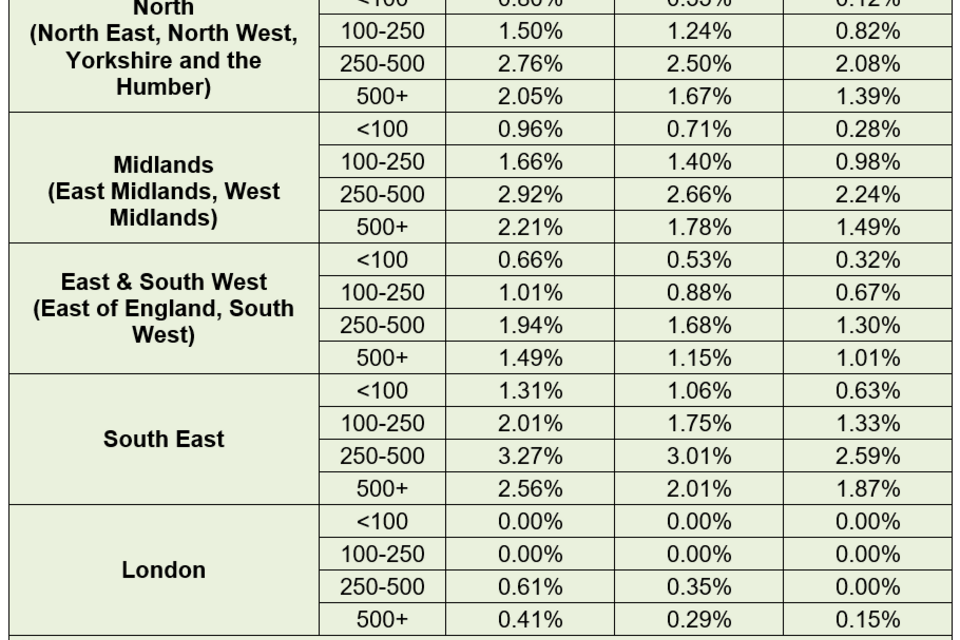
Step by step guide

G17. Once it has been confirmed that wider area impacts are relevant for the project, the following steps should be undertaken to monetise the impacts as part of the BCR calculation. Table 14 details the accompanying data sources which have been based on publicly available data. In some cases, the user may be able to justify using different data (e.g. local bespoke data, to estimate residential capital stock and value, which is acceptable if fully sourced).

1.) Identify the impact area

G18. The impact area should be initially identified as a 1.5km or 2.5km radius of the scheme, using the centroid of the site, and based on the constituent Lower Layer Super Output Areas (LSOAs).

G19. A variety of postcode/LSOA lookup tables are available online or from the Office of National Statistics (ONS) but where possible it is recommended that the impact area should be clearly mapped using Geographical Information Systems (GIS), to understand the area included.

G20. As a starting point, schemes below 1,000 units should use a 1.5km impact area whilst schemes over 1,000 units can use a 2.5km impact area but must include the 1.5km impact area as a sensitivity test. The 2.5km area should only be used if fully justified by local analysis of the impact area.

G21. A best fit LSOA approach should be used based on a population centroid approach, so that LSOAs where the majority of the population is located within the impact area are included. This should then be supplemented carefully by further analysis of the geography and local knowledge and consider excluding / including certain LSOAs where relevant, for instance:

Where the project is clearly unlikely to influence certain areas within the impact area. For example, a city centre scheme which incorporates a large element of the city centre that may be already regenerated, and the scheme is unlikely to have a significant impact.
Where there is a clear demarcation between an area and the site, for example a large park, river, or road, and the two areas are not closely linked.
Where the opposite may be true and the impact area appears too narrow given the importance of the scheme, for example a scheme that is transformational and will have a significant impact on a town’s image.

G22. The impact area should be clearly explained and justified, with careful analysis of the impact of including / excluding certain areas where necessary. This is particularly important for larger schemes when justifying the selection of the 2.5km impact area.

2.) Calculate the quantity of the existing residential housing stock

G23. The existing housing stock within the impact area should be calculated by using Valuation Office Agency (VOA) Council Tax: Stock of Properties data provided by LSOA, to identify the number of properties (by property type) in the footprint. Property types should include flats, terraced, semi-detached/bungalow and detached.

G24. The latest data should be selected to calculate existing stock as well as a comparison to 4 years ago to understand how stock has changed. For example, in 2022, the latest full year’s data on the housing stock will be 2021 and the comparison should be to the 2017 housing stock. This should not include any non-residential property.

3.) Calculate the rate of development

G25. The absolute growth in total units in the impact area over the last 4 years should then be calculated to identify the rate of development:

Low development – less than 4% growth.
Medium development – 4% to 12% growth.
High development – over 12% growth.

4.) Calculate the current stock value

G26. The current stock value should then be estimated by LSOA by property type. The Land Registry Price Paid database provides the most granular detail by location and property type and can be used to match sales values by type by postcode to LSOAs.

G27. In some instances (especially for detached properties) there are missing entries in the Price Paid data and the user will need to proxy the median price by type based on other values, for instance these could be the Middle Layer Super Output Area (MSOA), the surrounding LSOAs or if these do not exist the average LSOA or MSOA property price.

G28. Once the geographies are matched and sales values identified, the current stock value should then be estimated by multiplying the housing stock by type by median sales value by LSOA and summing the totals.

5.) Select an uplift factor

G29. Based on the rate of development (Step 3), the size of the scheme and location, select the relevant uplift factor as detailed in Table 12: Impacts table – % uplift to residential capital value within the impact area.

6.) Apply the uplift factor and calculate the gross impacts

G30. Multiply the current stock value by the uplift factor to calculate the gross economic gain.

7.) Incorporate impacts into the Cost-Benefit Analysis and adjust for additionality

G31. The gross wider area impacts should then be incorporated within the wider benefits of the economic appraisal, inputted in the correct price base, adjusted for growth in real terms GDP and discounted over time. Unless there is supporting evidence to suggest otherwise, the gross impacts should be inputted on a pro rata basis against the profile of units delivered.

G32. The gross wider area impacts should then be adjusted for additionality to derive the net impacts. This should consider both:

Deadweight in terms of the wider area impacts that would have occurred without the intervention. The default is for this to be based on the same assumptions as for the overall housing delivery, e.g. if 10% of the housing is delivered under the counterfactual, 10% of the wider area impacts should be counted as deadweight. In some cases, there may be strong justification to vary this, but this would need to be clearly set out.
Displacement in terms of the wider area impacts that would have occurred elsewhere from displaced housing activity. Prudently the default is to assume that displaced activity would have the same level of wider area impacts. Therefore, again, as a rule of thumb, it should be assumed that the displacement rate applied to the number of housing units delivered should also be applied to the wider area impacts.

G33. As an external impact, the wider area impacts should be included within the adjusted BCR.

8.) Sensitivity analysis

G34. Sensitivity testing should be undertaken, including to reflect project specific circumstances where local evidence is available.

G35. Alongside scheme specific sensitivity testing, particularly around the size of the impact area, it is recommended the following impact value ranges based on the rate of development category and unit numbers of the scheme should be applied, as shown in Table 13. These are based on the research findings regarding underlying development and location features. The sensitivity testing should apply the positive and negative percentage adjustment to discounted wider area impacts to understand how the BCR would change.

Table 13: Sensitivity analysis – impact value ranges

Number of units	Low Development (LD)	Medium Development (MD)	High Development (HD)
<250	+/- 5%	+/- 10%	+/- 15%
250 – 500	+/- 10%	+/- 15%	+/- 20%
500+	+/- 15%	+/- 20%	+/- 25%

Further adjustments and clarifications

Adjustments to reflect local circumstances

G36. The modelling upon which the guidance is based reflects the underlying profile of development schemes included in the original research. It is inevitable that circumstances will arise in which proposed developments are atypical and may exhibit significant characteristics that, based on detailed local analysis, could arguably provide wider area impacts above those recorded in the original research. In this situation, the above analysis should be undertaken to provide a baseline for discussion with an opportunity to introduce additional evidence as to local impacts. For example, the existing site may have very substantial negative externalities associated with them such as adverse visual and odour effects. The removal of these may well have a more significant placemaking impact than those identified through the impact factors in Table 12: Impacts table - % uplift to capital value above.

G37. In these atypical cases, a higher or lower impact rate should be applied based on local evidence, but the impact using the standard uplift rates shown in Table 12 should also be included in the appraisal as part of sensitivity testing. Strong evidence must be provided to apply a higher uplift than in Table 12.

G38. As outlined under Step 1, it may also be relevant to adapt the impact area to reflect the local market and scheme characteristics. This should be clearly set out and justified as well as presenting the values for the default radius impact area.

Option appraisal

G39. Due to the available sample data, the effects and therefore impact uplifts have been assessed for a broad range of unit outputs and thus it may be difficult to differentiate between options where, for example, all of them deliver over say 1,000 homes. In these cases, it is proposed that the placemaking impact is assessed for the largest option and that the appraiser then uses project specific evidence to adjust the scale of impact accordingly for each alternative option. As a rule of thumb, it is recommended that this is based on a pro-rata basis using the number of housing units.

Applying the impact model to a programme or multiple projects in the same local area

G40. There may be circumstances where a programme is proposed or there are multiple connected projects. Care will need to be taken not to ‘double count’ the wider placemaking impact. The appraiser will need to use local evidence to determine the most appropriate way to ensure that this does not happen. For example, it may be appropriate to model the impact area around a number of postcode/LSOA areas to reflect the broad spread of projects/programmes and then allocate the impacts on a pro-rata basis between individual projects.

Potential for double counting

G41. There will be potential for double counting with other external impacts that result in the wider area becoming more desirable. The following approach should be applied when considering other types of external impacts:

Amenity benefits – Section Giii provides an overview of how to estimate the external amenity benefits to the surrounding area of redeveloping brownfield sites. These benefits are likely to represent double counting if wider area impacts are included and unless there is significant justification otherwise, they should be excluded.
Transport benefits – if a scheme includes significant transport provision the appraiser should carefully consider the scope for double counting if including both transport and wider area impacts. This will depend on the nature and scale of the transport provision and who the ultimate beneficiaries are, with the scope for double counting likely to be highest where the transport scheme directly benefits the residents of the surrounding area. The appraiser would need to clearly identify and categorise the type of benefits arising from a scheme with housing and transport impacts and the best approach to monetising these, including any potential duplication^{[footnote 51]}.

Worked example

G42. A residential development will deliver 1,500 units on a brownfield site, on the edge of a city centre. The site has been stalled for decades and is causing significant blight issues, given its prominent gateway position. The remediation of the site will significantly improve the quality of the local environment. The housing to be developed is also critical for the sustainable growth of the city centre and will help transform the wider area in which it is located. The site will clearly have wider impacts on the surrounding area, which have been estimated as follows:

1) Impact area: the default impact area is identified as a 2.5km radius given the size of the scheme and all constituent LSOAs (using the population centroid method) are identified. Based on local knowledge of the area a final list of LSOAs at the 2.5km radius is identified.

2) Existing housing stock is calculated based on the final list of LSOAs by house type.

3) The rate of housing development based on growth over the last four years is identified as medium (between 4% and 12%).

4) The current stock value is calculated based on the median price by property type, and is approximately £7,000m.

5) An uplift value of 1.67% is selected based on location (North), rate of development (medium) and size (500+ units).

6) The gross placemaking benefit is approximately £116.9m.

7) Additionality is assessed as 60%, reducing the net impact to £70.1m.

8) The discounted placemaking benefit for the preferred option, once profiled in line with the housing and adjusted for additionality, is £44.4m. This is included in the adjusted BCR which moves from 1.0 to 2.1.

G43. Based on Table 13: Sensitivity tests, further analysis is performed with the gross wider area impacts ranging from £93.5m to £140.3m. The analysis above should then also be re-run at the smaller impact area of 1.5km as part of the sensitivity testing.

Data sources

G44. The accompanying data sheet to this guidance provides estimates of the residential capital stock values by LSOA across England based on the HM Land Registry Price Paid database and the VOA stock of properties data by property type. Where HM Land Registry Price Paid data by LSOA by type is missing (e.g. where no terrace homes have sold in a certain LSOA over the time period covered), the default is either the median MSOA or LA price by type (which can be sourced from House Price Statistics for Small Areas (HPSSA) data). Alternative data can be used but would need to be fully sourced and justified.

G45. The data sources are fully detailed below in Table 14.

Table 14: Data sources

Category	Data Source
Housing stock	Valuation Office Agency (VOA) Council Tax: Stock of Properties data (currently 1 April 2021 to 31 March 2022) (Table CTSOP 3.1), provided by LSOA. Total are used for Terraced, Flats and Detached Properties, whilst Bungalows and Semi-detached are combined.
House prices	Price Paid Data (PP), HM Land Registry, using the last available financial year (currently 1 April 2021 to 31 March 2022, to bring the stock value data into line with the VOA stock of properties data), provided by postcode. Alternative data sets, including to measure missing values: HPSSA, ONS, 2021. Note this only includes median price for all properties by LSOA (not by type) and MOSA.
Population Centroids	Lower Layer Super Output Areas Population Weighted Centroids, ONS, 2011. This data is used to identify the centroid of the constituent LOSAs within the impact area.

Gii Health impact of additional rented affordable housing

G46. There are both external impacts and private impacts associated with health improvements. To some extent, the (private) health impact is already captured in land value uplift which will reflect the private consumption benefits of additional rented Affordable Housing (AH). However, there are potential impacts not captured. How far they overlap – and therefore the extent to which they are potentially additional to the private health benefit – is discussed below.

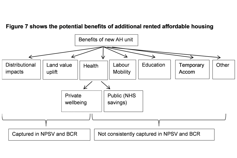
Figure 7 shows the different types of benefits that affordable housing offers which are captured with benefit cost ratios and those which are not currently captured.

G47. As the diagram above illustrates, there are a number of benefits associated with an additional rented AH unit. There is the private benefit – as measured by land value uplift which captures the efficiency benefit of converting land into a more productive use – and a potential distributional impact associated with the progressive nature of AH (see Annex H). Both these impacts are captured separately in an appraisal.

G48. However, there are also several impacts which are harder to monetise or are only qualitatively assessed in appraisals. These include fiscal savings from the potential savings on health care, improved labour mobility – increased housing supply lowers housing costs and therefore enables people to live in areas they might otherwise not be able to live – and potentially improved educational outcomes by reducing overcrowding. Finally it can result in savings to the exchequer from avoiding expensive temporary accommodation (TA) costs.

G49. This section focuses only on monetising potential health impacts. Assessing the potential significance of these impacts is problematic as these impacts are only likely to materialise if a new rented AH unit (a) enables a household to move away from a housing situation that was imposing an external cost and (b) another household does not then move into the same housing situation and instead this property is made either more habitable or could even be demolished (if the latter there may not be any land value uplift associated with the new rented AH unit as it would not be an additional housing unit).

G50. Therefore to estimate the potential health impact of additional rented affordable housing, the probability of a new tenant that had previously been living in a poor condition or overcrowded property needs to be calculated. In addition, as there are large negative health impacts from rough sleeping, an additional house that is allocated to a rough sleeper can be expected to deliver relatively large health impacts. This should be factored into the probability calculations.^{[footnote 52]}

Estimating probabilities

G51. To estimate the probability that a new tenant had previously been living in either poor or overcrowded conditions, the following working assumptions are made:

Within the social rented sector (SRS), it is assumed that those living in overcrowded accommodation are prioritised first;
10% of vacated properties are filled by a newly formed household (HH); and
1.5% of new lets go to rough sleepers (CORE data for 2019/20 shows around 1.5% of new lets to General Needs Private Registered Providers (PRP) are to those who say they were previously rough sleeping).

G52. The formula for estimating the probability that an additional dwelling reduces overcrowding is:

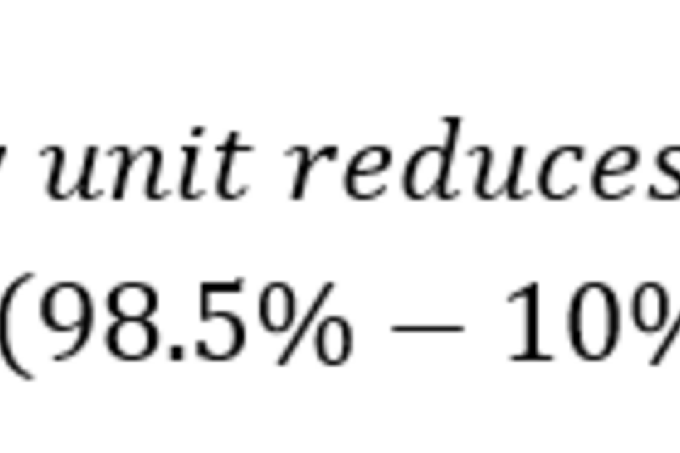
Where the 98.5% figure is derived from 100% less 1.5% of new lets going to rough sleepers.

Estimating the impact of poor housing on health

G53. The Building Research Establishment (BRE) has a model to estimate the impact of poor housing on the NHS. This is well-established and their work has been widely quoted, including by the World Health Organisation (WHO), National Housing Federation and Age UK. The BRE estimates the number of homes with Category 1 Housing Health and Safety Rating System (HHSRS) hazards and then estimates the cost to the NHS associated with them. There are 29 identified HHSRS hazards, including the risks from cold, damp, falls on stairs and overcrowding

G54. The study estimates the direct (medical) costs to the NHS that are likely to result from the presence of these hazards, using NHS data on costs of treating and caring for related health conditions up to a year following a health incident.

G55. The latest estimates from BRE for 2018 reveal that leaving vulnerable people in the poorest 11% of England’s housing costs the NHS over £1.5 billion per annum in first year treatment costs (in 2022 prices). The full report contains findings on the impact of all substandard dwellings and includes wider impacts on peoples’ life chances following a housing related incident, as well as the immediate medical costs. Initial estimates imply that the medical costs quoted above are at best 7% of the total cost of society. The methodology for estimating these is outlined in BRE’s 2016 report on the cost of poor housing.

G56. Table 15 shows BRE estimates of the impacts of different Category 1 hazards on NHS costs in a single year. It can be used to look at the savings to the NHS from removing Category 1 hazards through improving housing quality. For affordable housing it identifies the financial savings to the NHS from removing overcrowding as £149 per year (in 2022 prices).

Table 15: BRE cost estimates for 2018 (2022 prices)

Hazard	No. of Cat 1 Hazards	NHS annual saving if hazard fixed (£000s)	Per Unit Annual Saving (DLUHC estimate) (£s)
Excess cold	835,829	949,683	1,136
Falls on stairs	1,047,690	242,345	231
Falls on the level	409,643	115,261	281
Falls between levels	180,932	56,451	312
Fire	122,751	19,649	160
Collision entrapment	20,783	9,812	472
Falls – baths	8,265	2,547	308
Dampness	74,946	42,495	567
Hot surfaces	63,368	19,366	306
Lead	36,748	8,673	236
Entry by intruders	15,793	8,544	541
Radon	87,558	11,240	128
Sanitation (Personal hygiene)	17,629	4,068	231
Food safety	16,426	3,788	231
Pests (Domestic hygiene)	21,507	4,850	226
Overcrowding	36,879	5,508	149
Noise	4,893	2,650	542
Carbon monoxide	13,596	2,818	207
Structural collapse	8,848	1,518	172
Electrical problems	8,020	1,861	232
Ergonomics	10,015	2,344	234
Uncombusted fuel & gas	-	-	-
Lighting	-	-	-
Water supply	653	154	236
Excess heat	2,522	367	146
Explosions	-	-	-
Total dwellings with any Category 1 hazard	2,575,715	1,515,993	589

^{Note that:

1. The total sum of all dwellings with Category 1 hazards will be less than the sum of the individual hazards as some dwellings will have more than one Category 1 hazard.}

^{2. The total sum required to remedy all Category 1 hazards is less than the total number of Category 1 hazards multiplied by the average costs. This is because the modelling avoids the double counting of costs where repair work/energy improvements mitigate more than one hazard.}

Homelessness evidence

G57. Estimates for the typical per person cost of the health impacts of homelessness vary, as do estimates of the costs that remain even if they are housed.

G58. There is evidence on health costs for rough sleepers and for those with severe and multiple deprivation. Whilst we only account for the health benefits from rough sleepers here, some of the estimates used are for a broader definition of homeless than just rough sleepers, who may be expected to have higher health costs than other homelessness types which would mean these estimates may be an underestimate. There may also be additional health costs for other types of homeless people accessing social housing that could be considered on top of these.

G59. Estimates for the costs per person per year range from £2,300 to £21,900, with an average of around £8,700. Sources vary, from incidence rates and illustrative scenarios combined with unit costs, to survey data of particular interventions.

G60. Some of these costs are likely to remain even once someone is housed. We have considered two approaches for how to account for this. The first is to subtract the average cost of the general population’s use of the same health services, which is around £1,200 per person per year, suggesting a net saving on health of around £7,500. This is likely to be to an overestimate of the savings, as former rough sleepers may be expected to have more health problems than the general population.

G61. The second approach is to only count 27% of the gross costs as being avoided once the rough sleeper is housed, in line with Larimer and others (2009)^{[footnote 53]} which would give a net saving on health of around £2,300 per person per year in this case. This may be an underestimate of savings, as the source for the 27% estimate was a study of the chronically homeless with severe alcohol problems (whereas those rough sleepers accessing social housing are likely to have fewer problems than that group). Our working assumption is to take the average of the two approaches which gives a net saving on health costs of around £4,900.

Final calculation

G62. The formula for estimating the external health impacts from additional rented affordable housing is therefore:

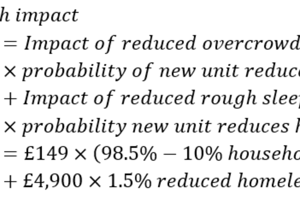
G63. Essentially the annual health impact is the annual £4,900 health care cost multiplied by the probability that someone is a former rough sleeper (1.5%) plus the probability of a new rented AH unit reducing overcrowding (88.5%) multiplied by the annual impact of reduced overcrowding from Table 15 (£149).

G64. Based on the above assumptions, the external health impact of an additional AH unit is equal to £206 per year or £3,900 in present value terms over 30 years. This value can be incorporated into the ‘adjusted’ BCR for each additional affordable or social rented house.

Giii Amenity cost of development on undeveloped land

G65. Estimates by consultants Eftec and Entec (PDF, 1.24MB) valued the external amenity benefits associated with different land types. The work involved a review of empirical evidence from 47 studies of amenity benefits using a range of willingness to pay and revealed preference methods. The estimates included values associated with recreation, landscape, ecology and tranquillity. These values can be used to estimate the loss of amenity benefits from development on different types of land.

G66. Estimates of the private land value uplift for greenfield land, for example those produced by the VOA, do not usually account for these amenity costs. If land value data does not account for amenity costs of development, the costs given in Table 16 below should be included in the appraisal and form part of the ‘adjusted’ BCR calculation.

G67. The real annual amenity benefits across different land types are shown below. These values are different to those in the Eftec and Entec report as they have been uplifted for GDP deflator inflation and so are in 2022 prices.^{[footnote 54]}

Table 16: Amenity loss values

Land Type	Amenity cost (2022 prices/ha)
Urban Core	119,258
Urban Fringe (Greenbelt)	1,963
Urban Fringe (Forested Land)	5,963
Rural	14,633
Agricultural (Extensive)	6,957
Agricultural (Intensive)	227
Natural & Semi-Natural	14,611

Amenity benefit of development

G68. Where a site is derelict or contaminated, it may have a potential environmental and amenity impact on local communities. Redevelopment of this land can provide an amenity benefit to communities, especially when new open and recreational space is created as part of the redevelopment. Where open space is created on previously developed land, the values in Table 16 can be applied as amenity benefits to society in the ‘adjusted’ BCR.^{[footnote 55]}

G69. Other methods that can be used to quantify and monetise amenity impacts are referred to within Annex A1 of the Green Book and discussed in further detail within the Green Book supplementary guidance on the Environment. This supplementary guidance includes the Enabling and Natural Capital Approach (ENCA) guidance and resources alongside the valuation of energy use and greenhouse gas emissions for appraisal guidance which provide detail on methods that may be applied.

G70. It should be noted that where placemaking regeneration impacts are estimated then the majority of amenity benefits are likely to be already counted in the placemaking impacts and so separate amenity impacts should not be estimated to avoid double counting.

Question 18

Annex H: Distributional impacts

Accepted Answer

H1. Annex A3 of the HMT Green Book makes clear that where a policy affects separate income groups differently distributional weights can be applied to provide a refined estimate of the policy’s impact on social welfare. (This analysis should be done in addition to unweighted appraisal of costs and benefits which is the minimum requirement of Social CBA.)

H2. The basis for distributional weights is the economic principle of the diminishing marginal utility of income. It states that the value of an additional pound of income is higher for a low income recipient than for a high-income recipient. The Green Book gives the example of a marginal utility of income of 1 which means that an individual with an income of £25,000 values an additional pound income twice as much as someone with an income of £50,000. A review of international evidence provides an estimate of the marginal utility of income at 1.3 which results in a faster decline in the value of an additional pound.^{[footnote 56]}

H3. The remainder of this annex:

Shows how distributional weights are derived from a utility function;
Provides a practical application of weights to a social housing tenure problem; and
Provides a practical application of weights to a local government funding problem.

H4. Further background on distributional weights is provided in the Green Book. This annex sets out an example on how distributional weights have been used in DLUHC appraisals and how the results of such analysis should be presented in an appraisal.

Theoretical derivation

H5. To calculate the distributional impact of a policy we first need to calculate the weights for individual income deciles. As noted above, the rationale for welfare weighting is based on the difference in marginal utility of consumption. The classic utility function is the logarithm function:

H6. In marginal terms:

H7. The marginal utility can be derived by dividing 1 by income, I, (which we use interchangeably with consumption) for each of the deciles:

H8. Distributional weights, (WW), can then be derived using the marginal utility of each decile (1/Id) as a percentage of average marginal utility (1/M):

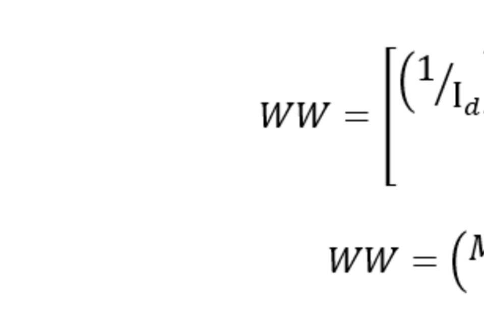
H9. However, the form of the utility function outlined above assumes the elasticity of marginal utility of consumption is equal to 1. More recent studies have shown different estimates of elasticity of marginal utility. The Green Book cites a review of international evidence which concludes that a reasonable elasticity value η is 1.3.^{[footnote 57]} This changes the form of the utility function (where U(C) = log(C) due to an assumption of η = 1) to:

H10. The marginal utility is therefore:

H11. This gives the following formula to calculate gross weights by income decile:

H12. This is the function adopted for the analysis of the social housing tenure problem below and the one that should be adopted more generally for distributional analysis of DLUHC interventions.

H13. The following calculation of distributional weights is illustrative. The use and calculation of distributional weightings should be viewed in the context of the rationale for the policy proposals being considered and whether they are suitable or not in that light. The HMT Green Book provides further guidance on this.

H14. Consider an intervention that benefits residents in the social housing tenure group. Using DWP data on median household income before housing costs, per decile, for all households^{[footnote 58]} in the UK gives the following gross weights per decile:

Table 17: Gross welfare weights by income decile (equivalised, disposable, before housing cost income)

Deciles	1	2	3	4	5	6	7	8	9	10	Median (M)
Income per week (Id)	204	307	376	444	512	582	665	771	928	1,363	547
Weight (M/Id)^1.3	3.60	2.12	1.63	1.31	1.09	0.92	0.78	0.64	0.50	0.31	1

H15. The gross weights vary from 3.6 to 0.31.^{[footnote 59]} For a person in the lowest income decile, a £1 benefit increases utility by 3.6 relative to the average marginal utility for all households, whereas for the highest decile, there is a marginal increase in utility of 0.31 relative to the average marginal utility for all households.

H16. The next step is to calculate an average weight for the policy based on the gross weights above. In this example, the intervention benefits residents in the social housing tenure group in England. To calculate the average welfare weight for tenants in the social housing tenure, the gross weights by decile are multiplied by the percentage of social tenants that are in that income decile. The distribution of social tenants (before housing costs) between income deciles of all households is as follows^{[footnote 60]}:

Table 18: Distribution of social tenants in England across UK income deciles

Income Decile	1	2	3	4	5	6	7	8	9	10	Total
% of social tenants	16%	19%	18%	14%	12%	9%	6%	4%	2%	1%	100%

H17. This shows, for example, 16% of social tenants are in the bottom income decile for all households.

H18. Multiplying the gross welfare weights for each income decile in Table 17 by the percentage of social tenants in that income decile from Table 18 gives the following weights:

Table 19: Gross welfare weight adjusted for housing costs

Deciles	1	2	3	4	5	6	7	8	9	10	Sum
Weight	0.58	0.40	0.28	0.19	0.13	0.08	0.04	0.03	0.01	0.00	1.75

H19. Summing across the income deciles in Table 19 gives an average weight for all social tenure households of 1.75.

H20. We then calculate welfare weights net of the cost to taxpayers (to reflect the negative marginal utility for households arising from paying taxes and other revenue raising activities). Thus, we subtract the £1 of transfer from the £1.75 benefit, leaving only £0.75 of pure welfare gain. In other words, spending £1 on a social housing tenant has an additional welfare equity effect of 75 pence on top of the direct £1 benefit which they receive from the spending.

H21. The Green Book recommends multiplying benefits by a welfare weight where appropriate, presenting the results alongside the unweighted benefits to demonstrate the impact of the weighting process. For business cases relating to affordable housing (and thus, social tenants), the rent subsidy that tenants would receive has been calculated as the difference between the affordable rent post-intervention and the market rent that would otherwise be charged on the home. In effect, this calculates the amount of additional money these tenants would have in their pocket compared to if they had to pay a market rent.

H22. In 2020/21, the average affordable rent on first-time let, general needs lettings was £142 per week^{[footnote 61]}. Given affordable rents are set at up to 80% of market rent for the home, we can infer the average market rent on affordable rent lettings to have been around £177, the difference therefore being £35 per week. The difference is funded by direct government subsidy.

H23. Assuming that the subsidy is distributed in accordance with the existing distribution of income of social tenants, welfare weights could be used to calculate the distributional benefit of the changes. This means multiplying £35 by 0.75, which gives a £26.25 benefit per week per tenant. If some of the rental subsidy resulted in lower housing benefit (and Universal Credit) expenditure as opposed to lower rents for tenants, further adjustments would be required to account for this.

Question 19

Annex I: VfM categories for initiatives which save money

Accepted Answer

I1. Some interventions result in financial savings to the public sector rather than increased spending. Examples include:

Invest to save spending, for example, on maintenance which reduces higher spend later on;
Reduction in service provision, for example, cutting back the coverage of a service or from reducing funding per person; and
Interventions which result in significant earned income from provision of services or involve the sale of assets.

I2. In such situations the present value of costs of the activity is negative. BCRs can no longer be used as summary measures of performance from monetised impacts as its size is no longer related to economic performance. In this case alternative measures for assessing VfM are needed.

I3. The general approach for initiatives which save public sector money is to use the Net Present Social Value, with a positive NPSV representing good VfM. Two positive NPSV scenarios are highlighted in Table 20 (represented by the green squares).

I4. Where the NPSV <0 , that is, the reduction in benefits are greater than the reduction in spend, the investment is likely to be poor VfM.

I5. Adjustments for non-monetised impacts - it should be noted that PVB and PVC represent only monetised impacts. Any non-monetised impacts should also be accounted for. If on balance non-monetised impacts are large in one direction it is possible that they will shift the NPSV from positive to negative or vice versa. If the shift is from negative to positive this implies that the intervention is VfM. Conversely if the NPSV shifts from positive to negative it implies the intervention is not VfM.

I6. Sensitivity testing – as before where there are uncertainties in the analysis and these are likely to be significant these should be tested.

Table 20: Value for money categories for money saving initiatives

Examples	Net Present Social Value	Impacts	Comments
1. Very High and Financially Positive VfM	NPSV >0.	PVB >0	Maintenance is often quoted as an example. Results in longer term savings and improved quality of service.
2. Economically Efficient Cost Savings	NPSV>0	PVB<0 but PVC fall faster than benefits	Decommissioning of a loss-making operation.
3. Poor but financially positive VfM	NPSV<0	PVB is more negative than PVC	Project fails to be VfM

Footnotes

The five “cases” or dimensions are the strategic, economic, financial, commercial and management dimensions. These are discussed in Chapter 2. ↩
Chapter 2 of the Magenta Book shows how to construct a logical chain process or theory of change. ↩
See also the DLUHC Evaluation Strategy. ↩
Social Cost-Effectiveness Analysis (CEA) is a variant of Social CBA which compares the costs of alternative ways of producing the same or similar outputs. Social CEA may sometimes be appropriate where: Wider social costs or benefits will remain broadly unchanged or for the delivery of a public good, such as defence; Output may not be proportionately quantified. For the majority of DLUHC interventions CBA is the best tool to use and so is covered in depth in this guide. Further guidance on CEA can be found in the HMT Green Book. ↩
Examples of corrective action to remove government failure might be removing a subsidy for production of a good which causes high levels of pollution or removing regulations which are overly onerous and lead to shortages of a good or service. ↩
The Net Present Social Value (NPSV) is the present value of the total stream of future benefits to UK society from a proposal less the present value of the total stream of future costs to UK society. ↩
It should be noted that not all measures set out in supplementary guidance enter the Initial BCR, e.g. reliability impacts from schemes which involve transport interventions are viewed as being more experimental than travel time impacts in Transport Appraisal Guidance. Users should carefully consider the advice on how to use impacts in supplementary guidance. ↩
In rows A and B a benefit may be positive or negative (in which case it is called a disbenefit). ↩
Note this includes estimates of land value uplift (see Chapter 4: Land value uplift approach to appraising development). ↩
A switching value refers to the changes in costs or benefits required to move an option into a different VfM category. They can be used to assess the stability of rankings where there are different options or the risks of an option being poor Value for Money. An example of the application of a switching value is given in Table 6. ↩
Even though evidence has not been monetised it is important that the assessment of magnitude and direction of impact is made using the most robust evidence available. The impacts assessed and evidence collected should be based on a well thought through theory of change. This should assess local context and could involve discussions with relevant subject experts. ↩
Note that costs are different from a disbenefit. Costs represent a use of public sector resources, disbenefits represent an impact on social welfare for example arising from an increase in carbon emissions. Costs may be upfront capital costs and/or costs from running a service. In some cases, an intervention will also result in savings or receipts to the public sector which should be netted off costs. ↩
For DLUHC spending proposals, the budget constraint should be real discounted net costs to the public sector. This means all exchequer costs should be accounted for when estimating net public sector costs. ↩
It should be noted that transfers – like Job Seekers Allowance, a government grant or Housing Benefit for example – are treated differently when calculating a BCR compared to the NPSV. For the BCR they represent a cost to government of the initial payment and so enter the PVC denominator. They also represent an equal and offsetting benefit to the recipient and enter the numerator. If an NPSV was used the transfer would net off to zero. ↩
Negative costs may occur because there are receipts or efficiency savings of sufficient size to offset initial public sector costs. As two examples, receipts might come from leasing of public property, whilst savings might come from new ways of working. ↩
The land valuation of a particular development will already account for the private costs (and possibly the benefits of potential government support) associated with a development as it is equal to the Gross Development Value of a site less any development costs less a minimum level of profit that is needed. Therefore, care should be taken to avoid double counting of costs (and benefits associated with government support). If the land value data accounts for all costs and the impact of any government support, then there is no need to separately account for further costs or the potential benefits to a firm from government support in the present value benefits. However, if the appraisal is using illustrative Valuation Office Agency land value uplift data, then this data will only account for ‘typical’ development costs. It will not account for any ‘atypical’ costs – such as those where there are large ‘clean-up’ costs associated with brownfield land for example – or the benefits of government support. These impacts will need to be accounted for separately in the appraisal. These ‘atypical’ private costs should feature as a negative number in the present value benefits as they represent a dis-benefit to the private sector. Any government grant or subsidised loan (less repayments) to the private sector should feature as a positive number in the present value benefits and as a positive number in the present value costs. ↩
As noted above, land value data may already account for the impact of a government grant or loan. If it does not, this should be included separately in the appraisal. ↩
Note that the assessment should be proportionate, reflecting the importance of the decision. How much resource is used to monetise impacts and assess risks and uncertainty is left to the judgement of the analyst making doing the appraisal. The focus of the appraisal should always be on investigating the costs and benefits relevant to the decision being made. ↩
These introduce additional granularity over the categories used in the 2016 DCLG appraisal guidance by breaking down both its Acceptable and High Categories into two separate categories. This allows improved assessment of VfM. ↩
This category would occur where an increase in expenditure results in negative benefits. ↩
It should be noted that the NPSV calculated in the example above will move from -£1m to positive with the introduction of the large non-monetised benefit. ↩
Monte Carlo Analysis is a simulation-based risk modelling technique that produces expected values and confidence intervals as a result of many simulations that model the collective impact of a number of uncertainties. ↩
Note that development costs are broken down into a number of elements including build costs, externals, sale and financing costs. Section B8 gives the full equation. ↩
In a competitive economy these are normal profits as there is no market power. ↩
Note this only holds where the value of the land in its new use is greater than its previous use. It is possible for a land use change to produce a negative uplift. ↩
For simplicity an inelastic supply curve is assumed. ↩
Consumer surplus is defined as the difference between the total amount that consumers are willing and able to pay for a good or service (indicated by the demand curve) and the total amount that they actually do pay. ↩
As noted above, land value uplift only covers private benefits to developers and buyers/renters of new property. It does not cover any external impacts which may arise from the development, e.g. wider area impacts, nor public sector costs in supporting schemes. These also need to be taken account of when measuring total welfare impacts from developments (see Annex B and Annex C). ↩
The change in consumer welfare for new property owners is equal to 0.5(Q2-Q1)(P1-P2). ↩
A useful definition of proportionality can be found in TAG. ↩
The two main structural economy models currently in use are Land Use Transport Interaction models and Spatial Computable General Equilibrium models. The former gives more local granularity in terms of changes in employment, residential and commercial activity including rents and prices. SCGE models are based on a much fuller representation of economic activity but the analysis tends to be at regional or higher level because of the amount of data required to set up the economic relationships in the model. A fuller explanation of the different model types is given in TAG Unit M5-3 supplementary economic modelling. ↩
Note this is the net effect once displacement and deadweight has been allowed for – see Annex D: Estimating additionality for further guidance. ↩
Consideration will also need to be given as to whether changes in land value are due to existence of transfers, e.g. the possibility that the land may benefit from tax-breaks. This could cause the value of the land to change but would represent a transfer from the exchequer to landowners. If the land value increases simply due to the existence of a transfer then this will need to be offset by an equal amount as transfers should have no impact on the NPSV. ↩
Although, the Green Book makes it clear that for an option to represent value for money it must also satisfy its strategic objectives. Longlist appraisal is mandatory and ensures options that don’t meet objectives are filtered out during the appraisal prior to shortlist analysis. ↩
The impact of firms moving to an area on the area they leave needs to be very carefully considered. It might be that there are significant adverse impacts from displacement, including on the local supply chain, employment and the physical and social fabric. ↩
In the Financial Case of a spending proposal, the OB adjustment should be excluded and instead a reasonable level of contingency should be made. This should be based on an assessment by the project team of risks allowing for identified activities to avoid occurrence and mitigate impact. When assessing risks, attempts should be made quantify the impact and probability of its occurrence. Techniques such as quantitative risk assessment could be used to assess contingency needed. For novel projects expert opinion may need to be brought in to support identification and measurement of risks. ↩
VOA data provides illustrative land value uplift estimates based on typical development costs. In this example, the estimated ‘clean up’ costs are considered atypical and so should be accounted for separately. ↩
In rows A and B a benefit may be positive or negative (in which case it is called a disbenefit). ↩
These are based on methods using established Green Book Principles, Green Book Supplementary and Departmental guidance. Where that guidance identifies a method as having a lower level of certainty because it is evolving it should go into Row B. An example of this would be agglomeration impacts in transport analysis. ↩
Note this includes estimates of land value uplift (see Chapter 4). ↩
These relate to impacts based on emerging techniques or where there is a high degree of uncertainty in the results produced by those techniques, e.g. amenity impacts. In some cases these will be discussed in supplementary guidance but be identified as being less reliable than other impacts. ↩
100% additionality has been assumed for the purposes of illustrating an AST. ↩
For simplicity, we have not included clean-up costs because of the corresponding DLUHC financial support which would cancel it out. ↩
39 x £200,000 = £7.8m. ↩
39 x £30,659 = £1,195,701. ↩
£7.8m - £1.2m = £6.6m = £6.4m discounted at 3.5% as recommended by the Green Book. ↩
Substitution – which is the replacement of one type of input by another type in response to an intervention is unlikely to be relevant for residential and non-residential interventions so is not discussed further. ↩
At the local level there are also likely be multiplier impacts relating to increased economic activity – these are covered in the Place Based Analysis Chapter. ↩
There are important distributional impacts from demand side interventions which need to be taken into account. For example, interventions might be targeted on extending home ownership to first time buyers or for less affluent families. ↩
Note that the ready reckoner does not apply to schemes which involve the provision of developer finance. ↩
This should be undertaken with reference to the levels of transport analysis as set out in Transport Appraisal Guidance (TAG) on wider economic impacts: TAG Unit A2.1: Wider Economic Impacts Appraisal, DfT, May 2019. ↩
We have concentrated on the impact of an additional affordable housing unit so have not accounted for the potential benefits of improving the condition of existing poor quality housing. ↩
Larimer, M.E., Malone, D.K., Garner, M.D. et al. (2009), ‘Health care and public service use and costs before and after provision of housing for chronically homeless persons with severe alcohol problems’, JAMA, 301(13): 1349-1357. ↩
They also include allowances for population growth and for income growth. Population growth means more people will be impacted on by changes in land type. Income growth increases people’s valuation of land type. ↩
Homes England, in collaboration with DLUHC, are working with consultants SQW and eftec to develop a framework and evidence base to improve the approach taken toward the assessment of environmental impacts within the economic appraisal of housing interventions. The framework will cover impacts related to land take, construction and the occupation of homes and will include the outputs from new research that aims to quantify the value associated with brownfield development through the use of discrete choice experiment methodology. ↩
Layard et al. (2008) “The marginal utility of income” Journal of Public Economics, Vol. 92, pp. 1846-1857, quoted in Annex 3 of the Green Book. ↩
HM Treasury (2022), Green Book, p 97, referencing: Layard eta al. (2008) “The marginal utility of income” Journal of Public Economics, Vol 92, pp. 1846-1857). ↩
DWP publish the data as part of the Household below average income series. The data is taken from HBAI 2019/20. ↩
For example, for a household in the lowest decile weekly income = £204. Therefore the weight = (547/204)1.3=3.6. For the top decile weekly income =1363. Therefore the weight = (514/1363)1.3=0.31. ↩
Based on DWP’s Households Below Average Income data, 2017/18 – 2019/20. ↩
Based on DLUHC’s ‘Social housing lettings in England, April 2018 to March 2019’. ↩

Cookies on GOV.UK

Applies to England

Foreword

List of abbreviations

DLUHC appraisal group

1. Introduction

The role of economic appraisal

Figure 1: ROAMEF model

Objectives of this guidance

The content and use of this guidance

Development of this guidance

Structure

2. The business case model

Introduction

The role of appraisal in the strategic and economic dimensions

Box 6 of HMT Green Book, Page 20: Logical Change Process

The rationale for intervention

Appraisal of options

Longlist appraisal

Option choices – broad description

Shortlist options appraisal

Options and the counterfactual

Assessing the impact of an option against the counterfactual

Example 1

Example 2

3. Assessing the Value for Money (VfM) of DLUHC interventions

Introduction

DLUHC appraisal summary table (AST)

Benefits

Table 1: Recommended DLUHC appraisal summary table

Costs

Net present social value (NPSV) and the benefit cost ratio (BCR)

Hypothetical examples of how to calculate the NPSV, initial and adjusted BCR

Example 1: A DLUHC grant to support a development

Example 2: A DLUHC loan to support brownfield land clean-up and development

Example 3: DLUHC will invest £20m to increase the number of polling stations to make voting more accessible to the public

Non-monetised impacts

Table 2: Qualitative assessment scale for non-monetised impacts

Value for money categories

Figure 2: Steps for deciding on a VfM category

Estimating VfM

Examining the impact of uncertainty on VfM

Types of uncertainty

Assessing uncertainty

Communicating VfM

Box 1: Examples of a value for money statement

Value for money statement example 1

Value for money statement example 2

Value for money statement example 3

Externalities

Box 2: Wider area impacts

Box 3: Examples of externalities

Example 1: externalities are of second order importance

Example 2: externalities are important but not fundamental to the case

Example 3: externalities are fundamental to the economic case

Natural capital

Greenhouse gases and climate change

Public service transformation, constitutional and social policies, and fiscal benefits

4. Land value uplift approach to appraising development

Introduction

Land value uplift explained

Accounting for external impacts

Using land value uplift in cost benefit analysis

Figure 3: Supply and demand diagram for residential floor space

Estimating the gross land value uplift impact from an intervention[footnote 28]

Estimating the net impact of an intervention

Estimating deadweight

Estimating displacement

Distributional considerations

Other issues to consider

5. The appraisal of place based initiatives

Introduction

Chapter aims

Structure

The role of place based analysis in appraisal

Proportionality

Robustness of analysis

Key questions

Issues in appraising place based initiatives

Links between strategic policy objectives and social welfare

Estimating the gross land value uplift impact from an intervention^{[footnote 28]}