The Rὺm model technical annex: assessing the impact of test, trace and isolate parameters on COVID-19 transmission in an October-like environment
Updated 19 February 2021

© Crown copyright 2021
This publication is licensed under the terms of the Open Government Licence v3.0 except where otherwise stated. To view this licence, visit nationalarchives.gov.uk/doc/open-government-licence/version/3 or write to the Information Policy Team, The National Archives, Kew, London TW9 4DU, or email: psi@nationalarchives.gov.uk.
Where we have identified any third party copyright information you will need to obtain permission from the copyright holders concerned.
This publication is available at https://www.gov.uk/government/publications/the-r-m-model-technical-annex/the-r-m-model-technical-annex-assessing-the-impact-of-test-trace-and-isolate-parameters-on-covid-19-transmission-in-an-october-like-environment
Abstract
In response to the COVID-19 pandemic, the UK government has implemented a large scale testing programme coupled with contact tracing capabilities and self-isolation support, NHS Test and Trace.
The programme aims to reduce transmission through testing to identify people who are infected, tracing their contacts (who are at heightened risk of being infected), and promoting self-isolation, both for confirmed positive cases and those they identify as contacts. Estimating the effectiveness of such a programme, defined as a reduction in R, is not possible though observational means as natural experiments are unavailable and designed experiments would be unethical.
Instead, we have implemented a probabilistic modelling approach (the Rùm model) to estimate the relative change in reproduction number in an October-like environment due to the combined effect of Testing, Tracing and Isolation (TTI) interventions. The model simulates individuals (tertiary cases) infected by the contacts (secondary cases) of an infected person (primary cases) and then calculates, by backpropagating using performance parameters for the NHS Test and Trace programme and parameterised epidemiological characteristics, what proportion of those simulated people would have avoided infection due to cases isolating on symptom onset or contact tracing. An October-like environment is defined to be one with symptomatic testing only, with contact tracing times distributed according to those in October, and behavioural and epidemiological parameters typical for October.
The model estimates that in such an environment the marginal impact of contact tracing would be a reduction in the R number by 1.7% to 4.6%. The relative effect of all TTI measures, including the effect of individuals self-isolating themselves upon experiencing symptoms, was estimated to be an R reduction of 18% to 33% (an absolute reduction of 0.3 to 0.6 with the assumption that R(October)=1.2). Hence, the majority of transmission reduction is due to isolation on symptoms. The model also estimates that if all NHS Test and Trace targets are met in an October-like environment, the marginal impact of contact tracing would reduce the reproduction number by 7% to 10%. The corresponding impact of all TTI interventions would be 33% to 43%, corresponding to an R reduction of 0.5 to 0.8.
1. Model description
The model assumes an infected population, whom we refer to as tertiary cases, and back-propagates through disjoint and independent transmission pathways to find the individual, secondary case, that infected the tertiary case and the individual, primary case, who infected the secondary case. As we only consider unique transmission chains, there is no explicit dependence in the model on the R0 number. As infection between cases is the outcome of interest in this model, the baseline counter-factual against which we compare, is a scenario in which individuals do not self-isolate on symptom onset and where no TTI programme exists.
We assign the probability that an infected individual is symptomatic as Ps. The event of symptom onset is only of interest in the primary and secondary cases. As we only assume symptomatic testing, we define the probability that an individual is tested as the symptomatic ascertainment rate (Pa), and we are only interested in the event that the primary case is tested.
We do not model test availability: we assume that if somebody requests a test, they are, eventually, tested. We do not consider the impact of a positive test on isolation: that is, we do not model the event that people don't isolate on symptoms, but do isolate on a positive test result.
We include 2 probabilities which describe compliance with isolation on symptoms: The first is the probability that an individual isolates on symptoms given that they request a test (Pit), and the second is the probability an individual isolates on symptoms given that no test is requested (Pint). The isolation event is successful if the individual isolated before onward infection occurred.
Only tested individuals provide contacts and a percentage of those contacts are infected and result in secondary cases, and a proportion of those are successfully contacted (Pc). A probability is assigned to the event that an individual isolates on contact (Pic), and contact isolation is successful if this isolation happens before the tertiary case is infected.
The overall success, or proportion of transmission that is averted, is calculated as the proportion of transmission chains that are broken as a result of any TTI intervention.
1.1 Notation of events
In the transmission chain, there are 3 potential events of interest:
• the event of infection
• the event of symptom onset
• the event of being contacted by test and trace
Because we neglect asymptomatic testing, and neglect the effect of self-isolation beginning only when a test result is received, we do not add to this list the event of receiving a positive test. The impact of this assumption is estimated to be small, as we assume that the majority of individuals who book a test will already be self-isolating on symptoms and the bulk of infectivity has likely passed prior to test result receipt. In this model, individuals only isolate on symptom onset or on contact.
In table 1, we provide the notation used to refer to these events for each case in the transmission chain.
Table 1: event notation
| Symbol | Description |
|---|---|
| S (i) | Time of symptom onset |
| I (i) | Time of infection |
| C (i) | Time when case contracted |
The superscript (i) denotes the case in the transmission chain for whom the event occurs. That is, (1) denotes the primary case, (2) denotes the secondary case and (3) denotes the tertiary case.
1.2 Parameter space
1.2.1 Parameterisation of epidemiological delay distributions
We define the epidemiological delay distributions as probability density functions used to describe stages of COVID-19 transmission. The probability that an individual isolates on time, to prevent onward transmissions, depends on when in the infectiousness curve they isolate. There is no exact method of representing the epidemiological delay distributions and so we explore two ways of representing the infectiousness curve in order to sufficiently capture this uncertainty.
Definition 1.1 (Incubation Period)
We define the incubation period as the time from infection of an individual to symptom onset, and parameterise this as follows (Zhang et al. 2020):
(1) S(i) − I(i) = f (τ ) ∼ Γ(α = 4.23, β = 0.81)
Definition 1.2 (Serial Interval)
The serial interval is defined as the time from symptom onset in the index case to symptom onset in the infected and parameterise this as follows (Zhang et al. 2020):
(2) S(i+1) − S(i) = g(τ ) ∼ Γ(α = 5.18, β = 0.96)
Definition 1.3 (Symptom to Onward Vector)
The symptom to onward vector, or infectiousness curve, is defined as the time from symptom onset in the index case to infection of the successive case:
(3) I(i+1) − S(i)
We present 2 methods for parameterising the delay between symptoms to onward transmission. Firstly, we can represent the symptom to onward vector delay as the difference between the serial interval and the incubation period:
(4) I(i+1) − S(i) = (S(i+1) − S(i)) − (S(i+1) − I(i+1))
To obtain the difference between the two probability distributions, we take the reverse convolution:
(5) I(i+1) − S(i) = h(τ ) = (g ∗ (−f ))(τ ) = ∫ (∞) (−∞) g(t)f (t − τ )dt,
where f and g are defined in equations (1) and (2) respectively. We assume, however, that onward infection cannot occur more than 2 days before symptom onset (He et al. 2020). This uses the same method as is presented by He et al. 2020. We will refer to this symptom to onward vector as the He curve.
The second symptom to onward vector is referred to as the Ashcroft curve (Ashcroft et al. 2020). One of the limitations of the first method, is that when the symptom to onward vector is convolved with the incubation period, it does not return the serial interval due to the truncation at 2 days before symptom onset. Ashcroft et al. 2020 aimed to consolidate this with the work of He et al. 2020. Instead of providing an analytic representation of the symptom to onward vector, the curve is fitted to observations and uses the incubation period as defined in Li et al. 2020. In Ashcroft et al. 2020, the curve represents infection to onward transmission, and so 5 days is deducted from the delay to retrieve the symptom to onward vector (assuming that the average incubation period is 5 days).
The effect of different symptom to onward vectors is something that can be explored in future work. However, these symptom to onward vectors are used to account for the sensitivity of the model to different epidemiological parameters. The Ashcroft curve can be viewed as a more pessimistic symptom to onward vector as a greater proportion of transmission occurs before symptom onset. The symptom to onward vectors are plotted in figure 1. Where the symptom to onward vector is less than zero, this corresponds to infection occurring before symptom onset.
Figure 1: Probability density function for the He and Ashcroft symptom to onward vectors
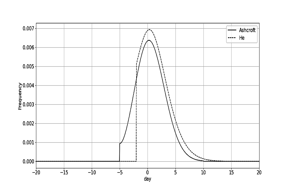
Figure 1 probability density
Definition 1.4 (Time to tertiary infection)
The time to tertiary infection is defined as the time from symptom onset in the primary case to infection of the tertiary case.
(6) I(3) − S(1) = S(2) − S(1) + I(3) − S(2) (7) = h(τ ) + g(τ )
All the above distributions are defined at hourly intervals, and interpolated if necessary, so that they are defined at the same granularity as the test and trace distributions.
Distributions can be added or subtracted by convolution. The distributions are padded with zeros where necessary in order that they match the same time range as the test and trace delay distributions and ensure convolutions are applied over the same time array.
1.2.2 Test and trace delay distributions
The end to end contact time is defined as the time from symptom onset of the primary case, to contact of the secondary case (or C(2) − S(1)). Where available, we used data from the test booking database and contact tracing database to construct the distribution of timings for each component of the end to end journey. The overall distributions used were created via random sampling of the distributions of the individual stages of a user’s journey, distinguishing between the different possible testing channels. The distributions of these individual stages were calculated based on data from October. Whilst this methodology does not follow a specific group of individuals through the entirety of the journey, it has the advantage of not relying on the joining of datasets.
The components of the Test and Trace contact tracing journey are:
• the time from symptom onset in an individual to booking a test. This is an unknown parameter, and the delay in days is assumed to be distributed according to Γ(α = 3, β = 1/2), truncated at 5 days. The mean was taken according to Kucharski et al. 2020.
• test booked to test taken. Taken from data.
• test taken to results communicated. Taken from data.
• time from results being communicated to results entering the contact tracing system. There is some limited data on this part of the journey which usually falls closely to 6 hours, so we set this part of the contract tracing time to 6 hours.
• time from case entering contact tracing system to case being reached and giving contacts. Taken from data.
• time from case giving contact to contact being reached. Taken from data.
All the above distributions are defined at hourly intervals.
The end to end contact tracing time is constructed as the addition of times for various parts of the contact tracing journey. In many cases this time distribution can be obtained directly from data internally available to NHS Test and Trace. In this case, we construct the distribution on the basis of data for the whole of England, provided by NHS Test and Trace.
The target contact tracing time is defined, as published in the NHS Test and Trace Business plan (Trace 2020), as a re-scaling of the October contact tracing time such that 80% of contacts are contacted within 72 hours from test booking. One possible route to achieving this target is laid out in table 2 (note that these are illustrative of one route to hit the overall end-end turnaround times, and are not in themselves individual targets). The October and target contact tracing distributions are plotted in figure 2.
Table 2: example target metrics
| Indicator | Illustrative future value |
|---|---|
| Time from ordering a test to taking a test | 100% within 48 hours, median 3 hours |
| Time from taking test to getting results | 80% within 48 hours, median 24 hours |
| Time from positive test result entering tracing system to reaching person who has tested positive |
85% within 94 hours, median 9 hours |
| Time from identifying to reaching contacts | 85% within 24 hours, median 15 hours |
Example target metrics for end-to-end contact tracing time that can be used to reach the overall target of 80% of contacts reached in 72 hours as detailed in the NHS Test and Trace business plan (Trace 2020)
1.2.3 Input parameters
In order to assess the effectiveness of the NHS Test and Trace programme, we compared the modelled performance of the system during the month of October 2020 to a counterfactual scenario. The month of October was chosen in order to be consistent with the reference month used in NHS Test and Trace's Winter Business plan (Trace 2020). It was also the last complete month of data at the start of the work. The counterfactual scenario imagines a world in which no testing takes place, infected individuals are not informed of their being infected and do not self-isolate upon experiencing symptoms. This scenario is, of course, unrealistic, however it is used here primarily as a control. The input parameters are defined in table 3. While epidemiological parameters are uncertain, we have no policy levers to control them. Behavioural and T&T parameters however, can be influenced by our decisions. A sensitivity analysis allows us to assess the impact of these parameters, and hence, observe the relative effect of particular aspects of the NHS Test and Trace system.
1.3 Mathematical description of the model
A transmission chain is stopped due to a secondary case isolating before a tertiary infection can occur. This can occur in 2 ways:
-
isolation on symptom onset in the secondary case
-
isolation on contact tracing of the secondary case
Figure 2: distribution for end to end contact tracing time.

Figure 2a distribution of the October end to end time
(a) Distribution of the October end to end time.
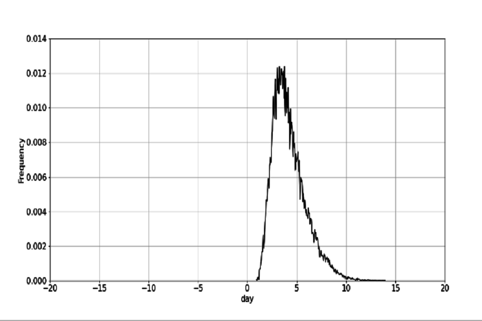
Figure 2b distribution of the target October end to end time
(b) Distribution of the target October end to end time.
Table 3: parameters and their descriptions
| Type | Symbol | Description |
|---|---|---|
| Epidemiological | P s | Assumed proportion of infections that are symptomatic. Is assumed to be 0.63. |
| T&T performance | P a | The total proportion of symptomatic infections picked up as cases |
| T&T performance | P s | Proportion of detected cases who are reached by CTAS |
| T&T performance | P s | Proportion of listed contacts traced and told to isolate |
| Epidemiological | P c3 | Proportion of onward infection who sit amongst listed contacts |
| T&T performance | P s | The percentage of cases that an individual infected that were successfully contacted. |
| Behavioural | P s | The probability an individual complies with isolation on symptoms, given that they ordered a test |
| Behavioural | P s | The probability an individual complies with isolation on being contacted. |
| Behavioural | P s | The probability an individual complies with isolation on being contacted. |
1.3.1 Symptom isolation
(8) P (isolation on symptoms) = Ps × Pa × Pit+ Ps × (1 − Pa) × Pint
(9) P (isolation is on time) = P (h(τ ) \> 0)
(10) P (tertiary infection prevented) = P (isolation on symptoms) × P (isolation is on time)
1.3.2 Contact isolation
(11) P (secondary contacted) = P (primary tested) × Pc
(12) = Ps × Pa × Pc
(13) P (secondary is contacted and isolates) = Ps × Pa × Pc × Pic
(14) P (secondary isolates on time) = P I(3) \> C(2)
(15) P (tertiary infection prevented) = P (secondary isolates on time) × P (secondary is contacted and isolates)
1.3.3 Joint distribution – considering both symptom and contact isolation of secondary cases
The probability of a transmission chain being stopped is the probability that it was stopped by either the secondary case isolating on symptoms, or isolating on contact, and doing so in time. This transmission reduction must be calculated in the same generation of cases.
The events of contact isolation and symptom isolation are not disjoint. The event of secondary symptom isolation includes the event that the symptomatic individual could also be a contact, and vice versa. Therefore:
(16) P (tertiary infection prevented) = P (tertiary infection prevented by symptom isolation)
+ P (tertiary infection prevented by contact isolation)
− P (tertiary infection prevented by symptom isolation ∩ tertiary infection prevented by contact isolation)
We derive the probability of the intersection in appendix A.1.
1.3.4 Impact of contact tracing alone
The impact of contact tracing alone is expressed as the additional impact of contact tracing on the proportion of transmission averted:
(17) Impact of contact tracing alone = P (tertiary infection prevented) − P (tertiary infection prevented by symptom isolation)
This neglects the possibility that a symptomatic secondary case could be contacted prior to onset of symptoms. Therefore, the impact of tracing alone is slightly underestimated.
2. Assumptions
In this section we outline the key assumptions that must be considered when interpreting these results. These also provide opportunities to further improve the model.
2.1 Structural assumptions and limitations
• We assume that symptom isolation happens exactly on symptom onset. There is a large degree of uncertainty in estimating the time after symptom onset that an individual isolates. This would largely need to be estimated from observational data or surveys, which are not likely to be very accurate. This, however, could be another parameter to be varied.
• We assume that contact isolation happens exactly on contact. Similarly to the above, there is a large degree of uncertainty in estimating when an individual isolates after contact.
• We assume no asymptomatic testing.
• The model is currently tuned to October levels of transmission (R0). R0 is implicitly represented in the parameter for percentage notified. We expect, that if prevalence increases, the percentage of contacts that are successfully reached would decrease.
• We assume that for those secondary cases who are both symptomatic and contacted by tracing, symptoms occur before contact. Therefore, a secondary case who develops symptoms and is contacted, would isolate on symptoms first given that they isolate on symptoms. This slightly reduces the impact of contact tracing, though the overall transmission averted would remain unchanged.
• We do not consider the possibility that the primary case could provide contacts, and continue to infect individuals if they don't isolate.
• We do not consider the time interval in which contacts were provided and how this affects the probability that they were infected. It is a requirement that contacts came into contact with the index case prior to the index case providing contacts.
This is implicitly accounted for by the percentage notified parameter, but this is a limitation that could be revisited in future work.
• Specificity and sensitivity are currently implicitly accounted for in the symptomatic ascertainment rate and so we don't explicitly account for the varying accuracy of PCR tests.
• We assume that the modelled transmission chains are all independent of each other. That is, each individual has different infectors. This assumption should hold in an October environment where the prevalence is low and where individual super spreaders aren't considered. However, as the prevalence increases, this assumption is less likely to hold.
• The incubation period and serial interval are estimated based on the original COVID-19 variant. In order to model any new Covid-19 variants, these distributions would need to be modified. We however do not foresee that any further changes would need to be made to the model. That being said, running this model with the new infectiousness curves should be done with care and understanding of the underlying assumptions of the model.
• We assume a homogeneous population.
2.2 Assumed parameter values
Table 4 summarises the central baseline parametric assumptions required in the model and the source from which they are based. These assumptions are set with regard to NHS Test and Trace operational data for October. We also summarise whether these parameters are varied. There are two ways in which these parameters can differ from their central October baseline value. Firstly, if there is uncertainty in the baseline estimate, the parameters are varied in baseline scenarios to capture low and high baseline October estimates. If this is the case, we say that baseline estimates are varied. Secondly, if the parameter can be controlled, for example if it is a T&T or behavioural parameter, then we can also define an aspirational target parameter value. If this is the case, then we say that it the parameter is controllable and are influenceable programme performance indicators or policy levers. Each parameter type is given in table 3.
Table 4: summary of parameters, their settings and the source for these assumptions
| Symbol | Is the variable varied or controllable? | Central baseline value | Justification |
|---|---|---|---|
| Ps | constant | 0.63 | Based on Ward et al. 2020 who use data from React2 serosurvey in England |
| Pa | baseline estimates are varied and is controllable | 0.63 | The proportion of cases identified is highly uncertain due to uncertainties in estimating actual COVID incidence at any point in time. Baseline assumption derived by assuming: 1) all cases detected were symptomatic (in practice 5% were non-symptomatic); 2) positive test detect 40% of all cases vs incidence estimates from the ONS infection survey, accepting that this comparison has limitations) (ONS 2020). |
| Pc1 | baseline estimates are not varied, but is controllable | 0.8 | Provided by NHS Test and Trace published statistics. |
| Pc2 | baseline estimates are not varied, but is controllable | 0.58 | Provided by NHS Test and Trace published statistics. |
| Pc3 | baseline estimates are varied, but as this parameter is epidemiological, it is not controllable | 0.6 | No direct data was available; expert judgement used on consideration of other data on contact patterns including CoMix (Jarvis et al. 2020). |
| Pc | Pc1 x Pc2 x Pc3 | 0.2784 | |
| Pit | baseline estimates are varied and is controllable | 0.8 | It is reasonable to assume that those who develop symptoms and request a test are both engaged with the system and have strong reason to believe they may have COVID. As both their engagement and potentially their strength of belief in having COVID may be higher than that of contacts (they have symptoms vs having been in contact with a positive case, but potentially not having symptoms), we believe their compliance with isolation should be stronger than for contacts. No clear evidence; expert judgement assumed at 80%. |
| Pint | constant - baseline estimate is not varied It is controllable, however, we do not define a target variable. |
0.2 | There is an argument to say that anyone who intends to isolate would get tested, as they are incentivised by the fact that if they test negative they can stop isolating. Taken to the extreme this might indicate 0% risk reduction. However it also seems plausible that some people would modify their behaviour even without seeking a test. No clear evidence, expert judgement assumes 20%. |
| Pic | baseline estimates are varied, and is controllable | 0.65 | NHS Test and Trace Isolation compliance survey suggests around 90% of those asked to self-isolate did not have any contacts during their isolation period. Assuming that 90% had a 100% reduction in transmission risk and the remainder had a 10% reduction in transmission risk would imply a 90% reduction in transmission risk overall. There will be an element of bias amongst those who took part in the survey so the actual reduction is likely to be less (although analysis of characteristics of those who participated vs those who didn’t showed no noticeable bias in characteristics of those who took part).In the absence of clear evidence, 65% is assumed. |
3. Results
3.1 Description of scenarios
To understand the impact of potential policy changes, we must consider the interaction of achieving policy targets with our uncertainties as to current performance. We consider four policy levers, and three different background scenarios against which these changes will have different degrees of influence.
We define the following as policy levers:
-
The proportion of symptomatic cases that are tested, or the symptomatic ascertainment rate
-
Compliance, as a combination of compliance on symptoms and a test result and compliance on contact
-
The end to end contact tracing distribution
-
The proportion of contacts that are traced
And for each parameter for which there is uncertainty in the estimate, we consider values describing estimates for current performance as:
• low
• central
• high
This range of values is chosen to represent the uncertainty in parameter estimates and are set based on a judgement of the level of uncertainty in the central baseline assumptions.
Against each of these three backgrounds, we then estimate the impact of each aspect policy-influenceable programme performance. For these, we consider the performance achieved in October, and a target value based on the NHS Test and Trace business plan.
For each of the low, central and high baseline parameter estimates, we model:
• October performance ('October')
• for each policy lever, re-model based on the target for that lever, with all other levers at the baseline October performance level
• performance if all policy lever targets are met ('All')
The policy lever values are given in table 5. We define Pint= 0.2 in all scenarios.
Table 5: policy lever values for range of estimates and the target scenario
| Parameter | Policy Lever | Low baseline | Central baseline | High baseline | Target |
|---|---|---|---|---|---|
| Pa | proportion symptomatic testing* | 0.52 | 0.63 | 0.7 | 0.8 |
| Pit | compliance | 0.70 | 0.8 | 0.83 | 0.85 |
| Pic | compliance | 0.57 | 0.65 | 0.80 | 0.8 |
| C(3) - S1 | contact tracing time | October E2E | October E2E | October E2E | Target E2E |
| Pc1 | proportion contacts traced | 0.8 | 0.8 | 0.8 | 0.9 |
| Pc2 | proportion contacts traced | 0.58 | 0.58 | 0.58 | 0.58 |
| Pc3 | proportion contacts traced | 0.5 | 0.6 | 0.675 | Same as baseline |
| Pc | proportion contacts traced | Pc1 x Pc2 x Pc3 |
*If a proportion of the population moves into the tested population, then we also assume that their isolation compliance increased from Pintto Pit.
3.2 Transmission averted by each scenario
We firstly present the transmission averted and impact of contract tracing alone as a result of using each representation of the symptom to onward vector, before combining these results to produce a range for estimated R reduction as a result of reaching the target for the different policy levers.
Table 6: transmission averted using the He infectiousness curve
Transmission averted using the He infectiousness curve, presented as the impact of achieving each policy target against a background of three different scenarios for October performance.
| Policy lever target | Low baseline | Central baseline | High baseline |
|---|---|---|---|
| October | 22.3% | 28.9% | 33.2% |
| Proportion symptomatic testing | 29.4% | 33.8% | 35.9% |
| Compliance | 26.4% | 30.9% | 34.0% |
| Contact tracing time | 22.8% | 29.7% | 34.4% |
| Proportion contacts traced | 23.6% | 30.9% | 36.2% |
| All | 39.4% | 40.9% | 42.0% |
Table 7: impact of Contact Tracing alone using the He infectiousness curve
Impact of Contact Tracing alone using the He infectiousness curve, presented as the impact of achieving each policy target against a background of three different scenarios for October performance.
| Policy lever target | Low baseline | Central baseline | High baseline |
|---|---|---|---|
| October | 2.0% | 3.1% | 4.6% |
| Proportion symptomatic testing | 2.8% | 3.6% | 4.9% |
| Compliance | 2.7% | 3.7% | 4.5% |
| Contact tracing time | 2.5% | 3.0% | 5.8% |
| Proportion contacts traced | 3.3% | 5.1% | 7.5% |
| All | 7.4% | 8.9% | 10% |
Table 8: transmission averted using the Ashcroft infectiousness curve
Transmission averted using the Ashcroft infectiousness curve, presented as the impact of achieving each policy target against a background of three different scenarios for October performance.
| Policy lever target | Low baseline | Central baseline | High baseline |
|---|---|---|---|
| October | 18.2% | 23.6% | 27.3% |
| Proportion symptomatic testing | 24.1% | 27.6% | 29.5% |
| Compliance | 21.6% | 25.3% | 27.9% |
| Contact tracing time | 18.7% | 24.4% | 28.5% |
| Proportion contacts traced | 19.3% | 25.3% | 29.8% |
| All | 32.7% | 34.1% | 35.1% |
Table 9: impact of Contact Tracing alone using the Ashcroft infectiousness curve
Impact of Contact Tracing alone using the Ashcroft infectiousness curve presented as the impact of achieving each policy target against a background of three different scenarios for October performance.
| Policy lever target | Low baseline | Central baseline | High baseline |
|---|---|---|---|
| October | 1.7% | 2.7% | 3.9% |
| Proportion symptomatic testing | 2.4% | 3.1% | 4.3% |
| Compliance | 2.3% | 3.2% | 3.9% |
| Contact tracing time | 2.2% | 3.5% | 5.2% |
| Proportion contacts traced | 2.8% | 4.4% | 6.5% |
| All | 6.8% | 8.1% | 9.2% |
The percentage of transmission that is averted as a result of the above scenarios due to isolation on symptoms or contact tracing are presented in table 6 for the He infectiousness curve, and table 8 for the Ashcroft infectiousness curve, and the impact of contact tracing alone is presented in table 7 for the He infectiousness curve and table 9 for the Ashcroft infectiousness curve.
3.3 Impact on reproduction number
The reproduction number (R) was estimated to be approximately 1.2 in October (Government 2020). This represents the baseline scenario where no policy levers are set to their targets. Therefore, we estimate the R number, in the absence of testing, tracing or self-isolating, to be:
R without any testing, tracing or self-isolation = Rbackground = 1.2
divided by 1 − transmission averted with no policy levers
(18) We provide a range of R numbers in a world without any testing, tracing or self-isolating to represent the range of estimates of the October baseline scenario. The estimated difference in R as a result of a policy intervention is therefore
(19) Rbackground − Rbackground(1 − transmission averted)
Combining the results from both the He and Ashcroft infectiousness curves, the transmission reduction as a result of TTI policies, ranges between 18.2% and 33.2%. Therefore, we estimate:
(20) RRbackground ∈ [1.4, 1.8]
The resulting estimated R reduction is presented in table 10. When interpreting these results, it is worth noting that these are calculated relative to an estimated October R number of 1.2. Therefore, these reduction estimates are dependent on the estimated R number and will be different if R is different.
Table 10: table presenting the ranges of estimates R reduction
Table presenting the ranges of estimates R reduction as a result of achieving the aspirational targets for various policy levers.
| Policy lever | Minimum R reduction | Maximum R reduction |
|---|---|---|
| No lever | 0.27 | 0.60 |
| Proportion symptomatic testing | 0.35 | 0.64 |
| Compliance | 0.32 | 0.61 |
| Contact tracing time | 0.27 | 0.62 |
| Proportion contacts traced | 0.27 | 0.65 |
| All | 0.48 | 0.75 |
4. Summary and conclusion
The effect of symptomatic isolation and test, trace and isolate interventions in October have been modelled using two different infectiousness curves and a range of parameter estimates in order to capture the uncertainty in both epidemiological estimates, and estimates of test, trace and isolate parameters. The impact of contact tracing alone is also estimated.
In October, the transmission reduction due to TTI interventions is estimated to be between 18% to 33%, with an impact of contact tracing alone of 1.7% to 4.6%. This is broadly in range with the Sage estimate for the impact of contact tracing of 2% to 4% (Ferguson and Green 2020). Using an estimate for R in October of 1.2 (Government 2020), this corresponds to a 0.3 to 0.6 reduction in the R number. If all targets for all policy levers are reached, the overall transmission reduction is expected to be 33% to 42% with an impact of contact tracing alone of 7% to 10%. Equivalently, estimating an October R0 number of 1.2, this would result in a 0.5 to 0.8 reduction in R.
Evidently, the effect of any policy lever on pessimistic estimates will be greater than that on optimistic estimates. However, the symptomatic testing rate has the greatest impact on transmission in both pessimistic and central scenarios.
The impact of contact tracing is relatively small. Even with small changes or improvements to the model, it is not expected that the impact of contact tracing will change drastically. It would remain of the same order of magnitude. Previous literature suggests that 44% (with a 95% confidence interval of 30% to 57%) of secondary cases are infected before symptom onset in the primary case (He et al. 2020). So 30% of transmission happens before symptom onset when using the He infectiousness curve, whereas 43% occurs before symptom onset in the Ashcroft curve, which is more in agreement with previous literature. Previous literature also states that, for a reproductive number of 2.5, contact tracing and isolation are unlikely to have a significant impact if more than 30% of transmission occurred before symptom onset, unless over 90% of contacts can be traced (He et al. 2020). More research would need to be done to conclude whether the same can be said for a smaller R number of 1.2, though our results do suggest that the same may be true. It also highlights the importance of recording contacts some time before symptom onset of the index case.
4.1 Future work
4.1.1 Introducing additional complexity
As we introduce further possible routes to isolation success, it increases the complexity of the arithmetic that describes the overall proportion of transmission averted. To illustrate, say we have the possibility that the transmission chain be stopped on symptoms, contact tracing or test result as a result of asymptomatic testing, and we denote these respectively as A, B and C.
The probability of infection of the tertiary case being prevented is therefore
(21) P (A ∪ B ∪ C) = P (A) + P (B) + P (C) − P (A ∩ B) − P (A ∩ C) − P (B ∩ C) + P (A ∩ B ∩ C)
As we add more events into the model, the complexity of this equation grows. Hence, in order to continue to develop further iterations of the model increasing in complexity in a scalable way, it would be necessary to create a class that automates the calculation of the above regardless of the complexity in the model.
4.1.2 Asymptomatic testing
Since October, testing levels have steadily increased. Moreover, asymptomatic testing (or mass testing) has also made up a larger proportion of overall testing. Therefore, in order to model the effect of TTI interventions post-October, asymptomatic testing will need to feature.
There are a number of additional epidemiological distributions that would need to be considered for asymptomatic testing. Firstly, the time to tertiary infection currently assumes symptom onset and so this would need to be reconsidered. Furthermore, as testing levels increase, more people are getting tested using LFD tests. The sensitivity of these tests depend on when in the infectiousness curve an individual is tested.
4.1.3 Household and non-household contacts
COVID-19 is more likely to spread between members of the same household than between different households. Furthermore, household members are more likely to be listed as contacts than non-household members. We can also assume that an individual is relatively likely to self-isolate when a member of their own household tests positive. So, even though household members are more likely to be contacted, and more likely to be contacted quicker, it may be the case that contact tracing is less effective on household contacts due to the possibility that they are already self-isolating. However, this should be explicitly modelled and estimates for compliance on these events such be justified.
4.1.4 Allowing for different COVID-19 variants
The model has been calibrated for the old COVID-19 variant. Whilst we believe it will be possible for the user to modify the epidemiological parameters to take into account the new variant, this will need to be done carefully before applying the model in 2021 circumstances. While we stand behind the structure of the model, the parameter values are now out-of-date, and further use of the model for policy, should only be done with careful re-calibration.
References
Ashcroft, Peter et al. (2020). COVID-19 infectivity profile correction. arXiv: 2007.06602 [q-bio.PE]
Ferguson, Neil and William Green (Nov. 2020). Private communication.
Government, UK (2020). The R number and growth rate in the UK
He, Xi et al. (May 2020). "Temporal dynamics in viral shedding and transmissibility of COVID-19", Nature Medicine 26.5, pages 672 to 675. issn: 1546-170X. doi: 10.1038/s41591-020-0869-5.
Jarvis, Christopher I et al. (2020). CoMix study - Social contact survey in the UK. Tech. rep. Centre for Mathematical Modelling of Infectious Diseases.
Kucharski, Adam J. et al. (Oct. 2020). "Effectiveness of isolation, testing, contact tracing, and physical distancing on reducing transmission of SARS-CoV-2 in different settings: a mathematical modelling study", The Lancet Infectious Diseases 20.10, pages 1151 to 1160. issn: 1473-3099. doi: 10.1016/S1473 to 3099(20)30457 to 6.
Li, Qun et al. (2020). "Early Transmission Dynamics in Wuhan, China, of Novel Coronavirus–Infected Pneumonia", New England Journal of Medicine 382.13. PMID: 31995857, pages 1199 to 1207. doi: 10.1056/NEJMoa2001316. eprint: https://doi. org/10.1056/NEJMoa2001316
ONS (2020). ONS Infection Survey, SPI-M (Oct. 2020). Private communication.
Trace, NHS Test & (2020). NHS Test and Trace business plan
Ward, Helen et al. (2020). "Antibody prevalence for SARS-CoV-2 in England following first peak of the pandemic: REACT2 study in 100,000 adults", medRxiv. doi: 10.1101/2020.08.12.20173690. eprint: https://www.medrxiv.org/content/ early/2020/08/21/2020.08.12.20173690.full.pdf
Zhang, Juanjuan et al. (July 2020). "Evolving epidemiology and transmission dynamics of coronavirus disease 2019 outside Hubei province, China: a descriptive and modelling study", The Lancet Infectious Diseases 20.7, pages 793 to 802. issn: 1473 to 3099. doi: 10.1016/S1473 to 3099(20)30230 to 9.
A Appendix
A.1 Derivation of the intersection of symptom isolation and contact isolation
We illustrate the events of isolation and isolating on time in fig. 3 for clarity. We should also note that A and B are independent from each other, as are D and F , therefore P (A ∩ B) = P (C) = P (A)P (B) and P (D ∩ E) = P (F ) = P (D)P (E).
Using the notation in figure 3, the event of interest is C ∩ F, hence
(22) P (C ∩ F ) = P (F )P (C|F)
(23) = P (F )P (A ∩ B|F)
(a) Diagram of the event of symptom isolation, where C denotes the event that tertiary infection was prevented. (b) Diagram of the event of contact isolation, where F denotes the event of that tertiary infection was prevented by contact isolation.
Figure 3: Venn diagrams illustrating the events were tertiary infection is prevent
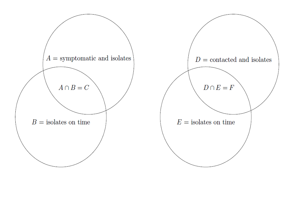
Figure 3 venn diagrams showing events if tertiary infection is prevented
The event A of being symptomatic and isolating is independent of event that contact isolation prevents tertiary infection, therefore,
(24) P (C ∩ F ) = P (F )P (A)P (B|F ) Applying Bayes' rule, we get
(25) P (B F ) = P (F |B)P (B) divided by P (F )
Substitution of the above, we get
(26) P (C ∩ F ) = P (A)P (B)P (F|B)
(27) = P (A)P (B)P (D ∩ E|B)
(28) = P (A)P (B)P (D)P (E|B)
(29) = P (C)P (D)P (E|B)
The requirement for secondary symptom isolation to occur on time (denoted by B) is given by:
(30) I(3) − S(2) \> 0
The requirement for contact isolation to occur on time (denoted by E) is given by:
(31) I(3) − S(1) \> C(2) − S(1)
However, as the time to tertiary infection is
(32) I(3) − S(1) = (S(2) − S(1)\ + (I(3) − S(2)\
there is a dependence on time from secondary symptom onset to tertiary infection.
Combing the above, we get
(33) P (C ∩ F ) = P (C)P (D)P (I(3) − S(1) \> C(2) − S(1)|I(3) − S(2) \> 0\
where P (C) is defined by eq. (10) and P (D) is defined by eq. (13).