CJRS final evaluation: Matched counterfactual analysis of employment outcomes technical note
Published 17 July 2023

© Crown copyright 2023
This publication is licensed under the terms of the Open Government Licence v3.0 except where otherwise stated. To view this licence, visit nationalarchives.gov.uk/doc/open-government-licence/version/3 or write to the Information Policy Team, The National Archives, Kew, London TW9 4DU, or email: psi@nationalarchives.gov.uk.
Where we have identified any third party copyright information you will need to obtain permission from the copyright holders concerned.
This publication is available at https://www.gov.uk/government/publications/the-coronavirus-job-retention-scheme-final-evaluation/cjrs-final-evaluation-matched-counterfactual-analysis-of-employment-outcomes-technical-note
Introduction
The Coronavirus Job Retention Scheme (CJRS) was an unprecedented intervention in the modern UK labour market. The scheme was designed to protect jobs, avoid permanent employer closures, help support household incomes, and reduce long-term damage to the labour market and wider economy. A total of 11.7 million jobs and 1.3 million employers were supported by the CJRS, with claims totalling £70 billion.
The matched counterfactual analysis estimates the impact of the scheme on jobs between November 2020 to April 2021. The approach described below is an extension of the empirical approach used in the CJRS interim evaluation, covering the entire duration of the scheme and supports the findings presented in chapter 4.2 of the CJRS final evaluation. It also includes an overview of the approach taken to calculate the cumulative impact of the scheme across its duration and alternative methodology considered to estimate the impact of the CJRS on jobs.
On the 31 October 2020, the CJRS was extended by a month up to the 2 December 2020. The cut-off date for the analysis was set on the day before the announcement, on the 30 October 2020, in-line with the approach taken in March 2020 for the counterfactual analysis presented in the interim evaluation. On 5 November 2020, the CJRS was extended further until March 2021, and later to April 2021. It should also be noted that in March 2021, the furlough scheme was extended further, to September 2021.
This analysis exploits the cut-off date to quasi-randomly assigns individuals to treatment and control group in the vicinity of 30 October 2020. New starters with a first employment declaration to HMRC on or before the cut-off date were eligible to be furloughed through the CJRS, but ineligible if this declaration was dated after the cut-off date. This analysis then compares employment trajectories for eligible and ineligible new starters near the cut-off date.
Findings indicate that CJRS claimants were more likely to remain employed between December 2020 and January 2021, however after January 2021, there is no significant difference in employment rates between groups. This may indicate the scheme’s impact on jobs reduced. Even so, the CJRS was effective in protecting jobs during the critical period of the second wave of COVID-19 between December 2020 and January 2021.
The cumulative impact of the scheme is calculated by adding together the peak jobs protected estimates from the March 2020 to October 2020 and November 2020 to April 2021 counterfactual analysis. Estimates for the counterfactual analysis for the period between April 2021 and September 2021 were not considered robust enough to include in the calculation of the cumulative impact. As noted in chapter 4.2 of the final evaluation, the expected impact of the scheme over this period would likely be small.
1. Empirical method
A matched difference-in-differences (matched DiD) approach is used. The approach used is consistent with the one detailed in chapter 2 of the CJRS interim evaluation – matched counterfactual technical note.
A matched approach is used to improve the balance between the control and intention-to-treat groups, as discussed below in more detail. This in turn allows more unobservable factors that might influence employment outcomes to be accounted for within the estimates.
2. Datasets
The analysis uses RTI submissions of new employments in October and November 2020, alongside HMRC CJRS admin data.
RTI submissions 1, 2 and 5-days around the cut-off were initially considered. The submissions closer to the cut-off date, such as those within 1-day, are viewed as being more robust as they reduce the chance of being impacted by changes in behaviour. However, a longer length of time around the cut-off date, such as a 5-day sample, increases the sample size used, which can improve the analysis.
The 5-working day sample between 26 October and 6 November 2020 has, in total, over 560,000 new employments. The primary estimate uses the 2-working day sample, which includes 186,000 individuals, of which approximately 63% were taken from the 2-days before the cut-off date and 37% in the 2-days after the cut-off date.
Although the sample used within the analysis is large, there are some important differences between the sample used and the whole furlough population. Some of these differences are discussed below in the limitations section. Table 2.1 outlines the differences in terms of age between the counterfactual sample and the total furlough population. Table 2.1 shows that in the counterfactual sample, there are approximately 10 percentage points more individuals in the 18 to 24 group and approximately 10 percentage points fewer individuals in the 50 to 64 group, relative to the total furlough population. This difference may impact the results of this analysis.
Table 2.1: Age breakdown of total furlough population and counterfactual sample
| Age | Total furlough population | Counterfactual sample |
|---|---|---|
| Under 18 | 2.7% | 5.6% |
| 18 to 24 | 16.4% | 26.9% |
| 25 to 49 | 51.6% | 52.2% |
| 50 to 64 | 23.7% | 14.3% |
| 65+ | 3.6% | 1.1% |
| Unknown | 2.1% | N/A |
Source: HMRC CJRS and PAYE RTI data
When assessing the 2 populations by gender, both groups have similar distribution which are around 50% men and 50% women.
Further comparisons of the 2 populations by additional variables used in the analysis, such as sector, region and scheme size, cannot be made. This is due to the differences in the way the underlying data is constructed.
Chapter 6 from the CJRS interim evaluation – matched counterfactual technical note outlines further details of the data sources.
3. Definitions
There are several stages to the analysis – matching and assessing balance in the sample, estimating the treatment effect through the DiD calculation, and scaling up the estimates to the CJRS population using a method that resembles an instrumental variable approach.
3.1 Assessing balance in the sample
Matching individuals improves the balance of observable characteristics between the control and intention-to-treat groups, facilitating the comparison of employment outcomes.
The compiled dataset contains monthly employment status, age, gender, pay, employment sector, pay frequency, migrant status, scheme size and region. These variables were chosen for 2 reasons: the first is the expected impact these variables have on eligibility for the scheme and employment outcomes. The second reason is the availability of these variables for the entire furlough population. The balance of the sample is assessed using a wide range of standardised methods. These include standardised mean differences, variance ratios, empirical CDF statistics, visual diagnostics, and prognostic scores.
Figure 3.1 shows an example of the improvement that can occur after matching. In this case, the matched variable is employment rates before the cut-off point and as shown, there is an improvement in each month, such as June 2020, where before the match there was a 5-percentage point difference between the control and intention-to-treat group. In September 2020, this difference is 8 percentage points. In both cases, the control and intention-to-treat groups match at 64 percent and 66 percent, respectively. It should be noted that the difference between the 2 groups pre-match is larger than when the same exercise was conducted for the analysis within the interim evaluation. Although there is a good balance post-match, the difference pre-match may have impacts on the final estimates.
This same approach was applied to several variables used in the analysis and improved the matching throughout.
Figure 3.1: Employment rates for the intention-to-treat group and control group pre-October 2020 before and after matching

Source: HMRC CJRS and PAYE RTI data
Table 3.1: Employment rates for the intention-to-treat group and control group pre-October 2020 before and after matching
| Month | Intention-to-treat | Control (matched) | Control (unmatched) |
|---|---|---|---|
| Apr 2020 | 66% | 66% | 61% |
| May 2020 | 65% | 65% | 59% |
| Jun 2020 | 64% | 64% | 59% |
| Jul 2020 | 64% | 64% | 58% |
| Aug 2020 | 61% | 61% | 55% |
| Sep 2020 | 66% | 66% | 58% |
The primary matching method used in the analysis is 1:1 nearest neighbour with replacement using propensity score matching (PSM). This approach uses a logistical regression to estimate the likelihood of an individuals in the control and intention-to-treat groups being eligible for the scheme, based on characteristics such as age, sector of employment and income.
The 1:1 nearest neighbour approach matched individuals across the 2 groups with similar estimated likelihood of scheme eligibility. Of the 186,000 individuals included in the matching sample, approximately 150,000 are matched. As the approach uses replacement, individuals in the control group can be matched multiple time to those in the intention-to-treat group resulting in 22,000 individuals in the control group matched to 128,000 individuals in the intention-to-treat group.
3.2 Estimating the treatment effect - matched difference-in-differences
Once the most suitable matched sample is achieved, the DiD regression is run. The matching process determines individual weights in a way that balances the sample, and those weights are considered when running the regression.
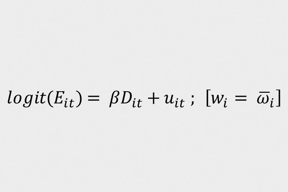
The following model is used:
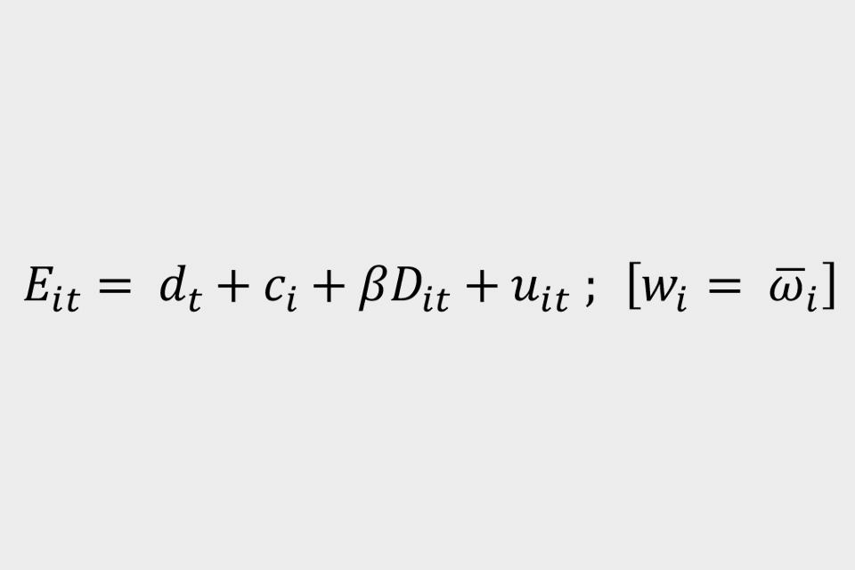
where employment status ‘E(it)’ takes 1 if individual ‘i’ is in paid employment in month ‘t’ and zero otherwise. The parameter ‘beta’ is the key parameter and measures the differences in employment rates between those in the control and intention-to-treat groups before and after the cut-off date. The difference in employment rates after the cut-off date is assumed to be due to CJRS eligibility and thus gives the impact of the scheme on jobs. This parameter is derived from the binary variable ‘D(it)’ which takes one if individual ‘i’ is in the treatment group after November 2020, and zero otherwise. The specification includes individual fixed effects ‘c(i)’, monthly fixed effects ‘d(t)’. Individual weights are given by the vector ‘Wau-bar(i)’. The error term is given by ‘u(it)’. This is termed as equation (1).
Figure 3.2 illustrates the results from the analysis. It shows a good match in the employment rates between the 2 groups pre-treatment, suggesting the groups are comparable. After which, there is a divergence in employment rates in December 2020 and January 2021, which is assumed to be due to the impact if the CJRS. The difference is an estimated 1.5 percentage points in January 2021, the biggest gap, before converging to an employment rate of 90%. After this point, the gap diverges again by approximately 1 percentage point, indicating the diminishing impact of the scheme, however as flagged below, these figures are not statistically significant.
Figure 3.2: Proportional employment rates for the intention-to-treat group and control group from April 2020 to April 2021

Source: HMRC CJRS and PAYE RTI data
Table 3.2: Proportional employment rates for the intention-to-treat group and control group from April 2020 to April 2021
| Month | Control | Intention-to-treat |
|---|---|---|
| Apr 2020 | 66% | 66% |
| May 2020 | 65% | 65% |
| Jun 2020 | 64% | 64% |
| Jul 2020 | 64% | 64% |
| Aug 2020 | 61% | 61% |
| Sep 2020 | 66% | 66% |
| Oct 2020 and Nov 2020 | 100% | 100% |
| Dec 2020 | 97% | 98% |
| Jan 2021 | 93% | 94% |
| Feb 2021 | 90% | 90% |
| Mar 2021 | 89% | 88% |
| Apr 2021 | 83% | 82% |
It is difficult to draw robust conclusions with the available evidence on why the groups converge, as illustrated in figure 3.2. There could be several potential reasons, as outlined in chapter 4.2.2 of the CJRS final evaluation, including improvements in the broader labour market as economic uncertainty eased. This would reduce the number of individuals in the control group becoming unemployed causing the convergence. Similar trends were observed within the counterfactual analysis spanning the period April 2020 to October 2020 presented in the interim evaluation.
It should be noted that only the estimates for December 2020 and January 2021 are statistically significant, both at the 5% level. Testing the estimates for February, March and April 2021 show they are not statistically significant, meaning it cannot be concluded that the differences between the 2 groups are being driven by the impact of the CJRS, however the figures are presented for completeness.
There are 2 potential sources of bias when using a linear probability model to calculate the DiD estimator:
- unconstrained estimators – using a linear probability model may allow estimates to move beyond or below the natural bounds of a probability (i.e. below 0% and above 100%)
- functional form – a linear probability model only calculates a constant impact/change along the gradient of the line plotted and may not account for variations in effect that might occur when moving along the probability distribution. For example, different ages may be associated with higher or lower chances of being in employment / unemployment
In response to the first source of bias, evidence from the literature suggests this is only problem when using linear probability models for forecasting or calculating predictive probabilities. When estimating the causal effect of a treatment on an outcome, as is done in this approach, the risk of bias is reduced[footnote 1]. Additionally, by using a binary independent variable, alongside weighting the regression, the estimates are more likely to be constrained.
In response to the second point, the functional form is not an issue as the DiD term, the variable of interest in the equation, only takes on 2 values (0 or 1)[footnote 2]. This helps mitigate against the issue of the variables not having a consistent impact.
To help further mitigate these concerns, an alternative methodology producing a secondary estimate of the scheme’s impact on employment outcomes is specified in the Alternative Methodology – Logistic Regression section below.
3.3 Scaling up exercise
The estimates derived from the DiD regression are scaled up to the broader CJRS population using the Wald Estimator. This is consistent with the approach used in the interim evaluation and more details can be found in chapter 3 of the CJRS interim evaluation – matched counterfactual technical note.
This approach builds on the scaling up exercise used in (Autor, et al., 2020)[footnote 3] and (Bishop and Day, 2020)[footnote 4]. Equation (1) gives the effect of CJRS worker eligibility criteria on employment. To estimate the effect of receiving the CJRS on employment, the analysis considers the probability of the CJRS claims coming from both control and intention-to-treat groups.
To understand this, consider that if 100% of intention-to-treat individuals took up the CJRS and 0% of control individuals, then the impact of the CJRS on employment would be equal to the impact of eligibility on employment. However, this is not true, so the analysis must scale the estimates accordingly.
The analysis scales up the estimates using the Wald estimator[footnote 5]. The impact of the CJRS on employment rates is given by:
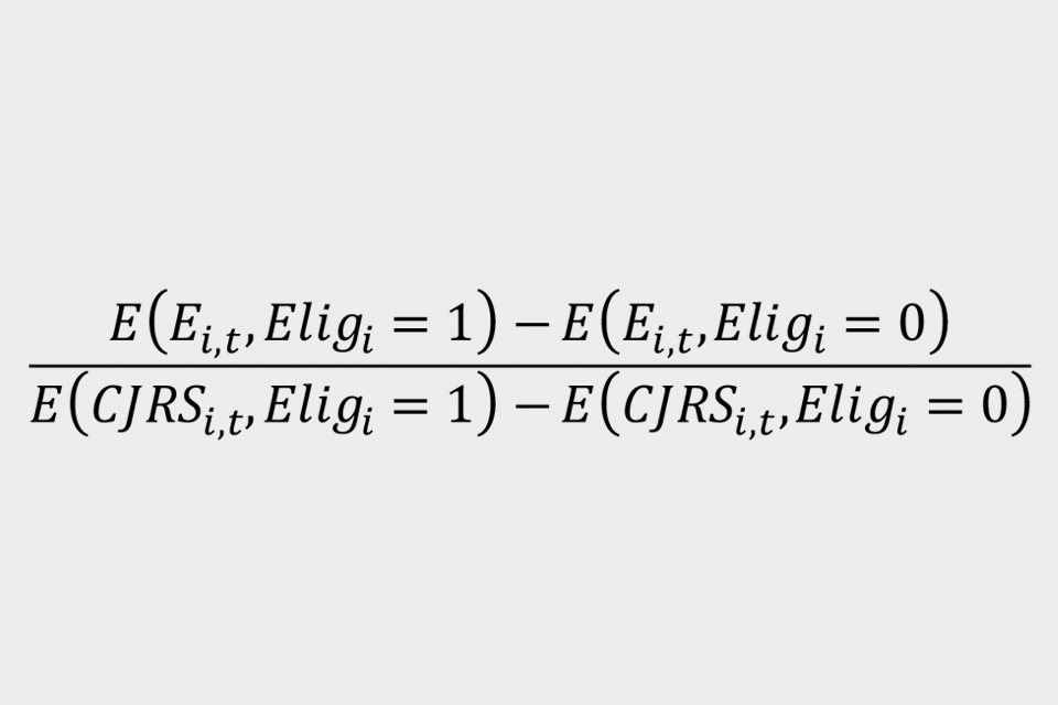
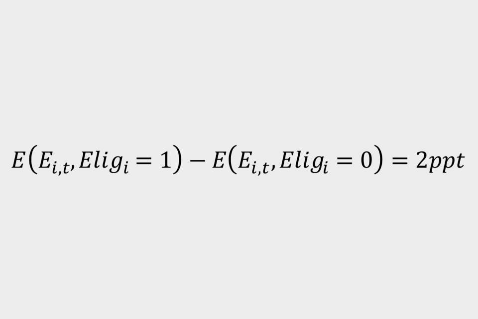
Where ‘E(i,t)’ indicates PAYE employment for individual ‘i’ in month ‘t’ and ‘CJRS(i,t)’ indicates take up of the CJRS for that individual. This is termed as equation (2). The numerator gives the likelihood that an individual is employed in the intention-to-treat group compared to the control group in January 2021:
To estimate the 2 probabilities in the denominator, use the proportion of the intention-to-treat group who are on furlough in the period October 2020 to April 2021 as the probability of receiving the CJRS for treatment individuals:
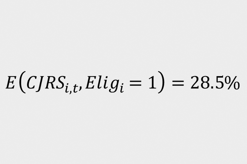
Similarly, for control individuals use:
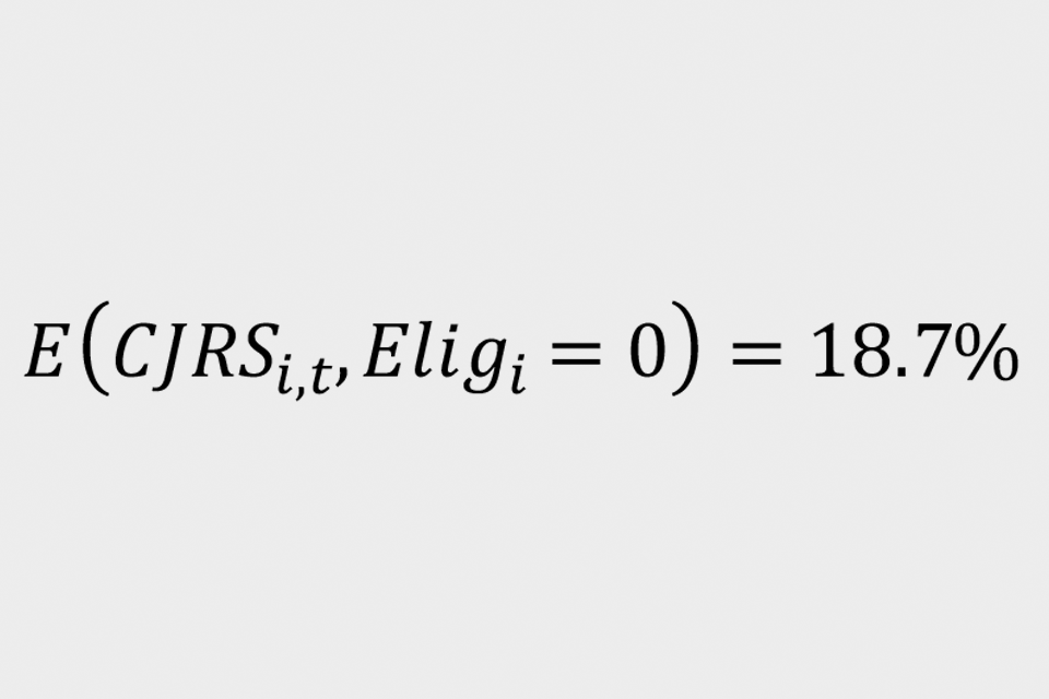
Thus, the average difference in scheme take-up rates between the intention-to-treat and control groups is approximately 9.8 percentage points.
The scaled-up figures are bounded by unique furloughs between October 2020 and April 2021, which relate to approximately 1.9 million individuals.
Table 3.3 below shows how the January 2021 scaled figured is calculated using the Wald estimator approach. Once scaled, estimate approximately 300,000 jobs were protected.
Table 3.3: January 2021 scaling up calculation
| Column | Variable | Value |
|---|---|---|
| A | Average difference in furlough take-up | 10% |
| B | Unique furloughs | 1,900,000 |
| C | Jan-21 employment rate difference | 2% |
| D | Scaled-up employment rate (C / A) | 16% |
| E | Scale up jobs protected (D * B) | 296,254 |
Source: HMRC CJRS and PAYE RTI data
3.4 Estimating the cumulative effect
The cumulative effect of the scheme is calculated by adding together the jobs protected estimate derived from the methodology described above. The peak jobs protected months – May 2020 and January 2021 – from the 2 versions of the analysis are added together to calculate the final cumulative impact.
This approach exploits the use of unique furloughs when scaling up the counterfactual estimates. By using the impact on unique furloughs, the risk of double-counting jobs protected across the 2 versions of the counterfactual analysis is greatly reduced. However, this may also lead to an underestimate of the final jobs protected estimate. The final figure is bounded by those unique furloughs between November 2020 and April 2021, so only includes individuals who were put on furlough between these 2 months. Therefore, the final scaled-up figure does not include those individuals who were already on furlough before the cut-off point, that being individuals placed on furlough between the beginning of the scheme and October 2020.
Estimates from the counterfactual analysis show that 3.4 million jobs were protected in May 2020, whilst 300,000 jobs were estimated to have been protected by the scheme in January 2021.
This gives cumulative jobs protected estimate of 3.4 million plus 300,000, which is equal to 3.7 million jobs protected. How this is calculated is shown in table 3.4.
Table 3.4: Cumulative jobs protected of the CJRS calculations
| Column | CJRS period | Jobs protected |
|---|---|---|
| A | May 2020 jobs protected | 3,400,000 |
| B | January 2021 jobs protected | 300,000 |
| C | Cumulative jobs protected (A + B) | 3,700,000 |
Source: HMRC CJRS and PAYE RTI data
3.5 Alternative methodology - logistic regression
After critically assessing the primary jobs protected estimate derived from the linear probability model (LPM), an alternative approach using a logistic regression model was specified. Two logistic models were considered: a conditional logistic model and a weighted logistic model.
After carefully considering the strengths and weaknesses of both estimates, it was decided the outputs from the weighted logistic regression would form the report’s secondary DiD estimate.
Although the conditional logistic model can incorporate group fixed effects, it was challenging deriving the monthly impact of the CJRS using this approach. Additional limitations, both conceptual and practical, led to the decision to trial the weighted logistic model, given by equation (3) below:
The weights are derived from the same process as those given in the LPM. The coefficient ‘Beta’ represents the log-odds of the difference of employment outcomes of the intention-to-treat group divided by odds of the difference of employment outcomes of the control group. ‘D(it)’ represents is the DiD interaction term, ‘u(it)’ represents the error term and ‘E(it)’ is the model’s binary dependent variable, taking the value of 1 for employed or 0 for unemployed.
4. Results
Taking the exponent of estimate ‘Beta’ allows us to find the odds ratio for each month as seen in the table 4.1 below.
Table 4.1: Outputs from the weighted logistic regression estimating the impact of the CJRS on employment outcomes between December 2020 and April 2021
| Month | Estimate | Standard Error | Statistics | P-value | Odds Ratio |
|---|---|---|---|---|---|
| Dec 2020 | 2.07 | 0.02 | 104.20 | 0.00 | 7.92 |
| Jan 2021 | 1.02 | 0.01 | 80.21 | 0.00 | 2.78 |
| Feb 2021 | 0.45 | 0.01 | 42.95 | 0.00 | 1.56 |
| Mar 2021 | 0.27 | 0.01 | 27.70 | 0.00 | 1.31 |
| Apr 2021 | -0.21 | 0.01 | -24.59 | 0.00 | 0.81 |
Source: HMRC CJRS and PAYE RTI data
The odds ratio is a relative measure of association. It tells you how much more likely an outcome is in the intention-to-treat group compared to the control group. The odds ratio being greater than 1 suggest that the intention-to-treat group had a relatively better outcome than the control group.
Table 4.1 shows that in the month of December 2020, an individual in the intention-to-treat group had 7.92 times higher odds of being in employment relative to those in the control group. There is another strong, positive impact of those in the intention-to-treat group in January 2021 before a reduction in impact in the months leading up to April 2021, shown by the odds-ratio moving closer to 1. This trend is similar to the LPM estimates where the jobs protected peaked in December 2020 and January 2021. Then the impact of the CJRS diminishes each month until it is less than 1 in April 2021.
4.1 Discussion
As outlined above, there are several potential problems that can bias the estimates from the LPM. The unconstrained estimator can push the probability of an individual being in employment above 100%, which can lead to an overestimate of the scheme’s positive impact. The problem of functional form can lead to the incorrect specification of a variables impact when that impact is not consistent. Using a logistic regression approach helps mitigate against these issues.
The characteristics of a logistical regressions ensure the estimates are bounded between 0 and 1, ensuring they do not suffer from bias associated with unconstrained estimators. Additionally, a logistic model can account for differences in effect at different variable levels as it does not rely on a consistent impact, mitigating issues of functional form associated with the LPM.
Even so, due to the nature of odd ratios, only the relative strength between the intention-to treat group and the control group can be calculated. Using a logistic model carries extra complexity in terms of interpretation of the estimator and application to the Wald-Estimator. This means that there is not a scaling up exercise to calculate the number of jobs protected by the CJRS, making it difficult to interpret and draw a tangible figure of jobs protected by the CJRS for policy evaluation.
Applying a logistic regression approach avoids these 2 issues, which in turn can help assess to the extent these issues might be impacting the jobs protected estimate derived from the LPM. Comparing the overall trends between the LPM and weighted logit model shows they are similar. Both approaches indicate most jobs were protected in December 2020 and January 2021 and then number of jobs protected by the CJRS diminishes each month, building further confidence in the LPM estimates.
5. Additional information
5.1 Limitations
The limitations of the analysis remain consistent with those included in chapter 5 of the CJRS interim evaluation – matched counterfactual technical note and are summarised below.
Factors which cause downward pressure on the estimates include:
- This method does not fully estimate the number of jobs protected where the employer would otherwise have ceased trading. The estimates reflect this to the extent that employers most likely to cease trading are expected to be most likely to make redundancies amongst their ineligible employees. However, this estimate does not capture the impact of CJRS support in helping businesses to keep trading when the business would have otherwise ceased trading and thus protected other non-furloughed employments who would have become unemployed.
- This analysis does not include wider macroeconomic impacts of the CJRS, such as supporting business investment or household spending that may have also supported jobs indirectly. For example, those who became unemployed may have been able to find new employment more easily due to the CJRS supporting other employments and being likely to have provided a fiscal stimulus, therefore preventing a higher number of individuals in unemployment at the same time.
- There will be some spill-over of effects between the treatment and control groups as larger employers may have been able to shield ineligible new employees from redundancy, as they have benefited from the CJRS support for their eligible employees. For example, evidence from the employer qualitative research indicates some employers were able to use the CJRS to support internal finances and consequently retain non-furloughed employees.
Factors which cause upward pressure on the estimates include:
- Where employers were going to make redundancies without the CJRS, these may be more likely be from their newer employees.
Limitations in the data:
- The cut-off date used in the analysis for employments is not perfect in practice. It is difficult to precisely identify when a new employment began. Furthermore, individuals may have had second jobs and there was a level of error and fraud.
- Related to the above point, in the sample of new employments in HMRCs RTI data, it is not possible to accurately isolate transfers (movements between PAYE schemes for the same employer) from new employments. This equally effects both the control and intention-to-treat group and suggests some individuals in the control group may in fact have been eligible.
Limitations in generalising beyond the sample:
- There are limitations with generalising the findings to the whole CJRS population, as the scheme may have different impacts across different employee characteristics. The analysis is only able to use new employments due to the identification strategy. The distribution of characteristics, such as PAYE scheme size and sector, is not identical to the full User population.
- An additional consideration is the timing of the cut-off, on a Friday at the end of the month. There is some evidence that individuals who are included in filing later in the month and at weekends may have different characteristics to the wider population, which is broadly reflected in the difference between the intention-to-treat group and control group pre-match, as shown below in figure 5.1. However, the matching approach tries to alleviate these concerns.
- Relative to the estimates presented in the interim evaluation, there is a higher chance the results from this counterfactual analysis may be impacted by anticipatory behaviour, creating bias in the estimates. There would have most likely been widespread employee and employer knowledge of the furlough scheme, which could have led to changes in behaviour. This type of behaviour is difficult to account for in the estimates and may impact the results.
5.2 Robustness analysis
The first check involved using the baseline DiD. The population from the 2-day sample is used, however individuals in the control and intention-to-treat groups are unmatched. Figure 5.1 shows the impact of not matching across the groups before the cut-off point in October / November 2020, where in September 2020 there is an 8-percentage point difference in employment rates. This contrasts to the trends shown in figure 3.2, where the matching improves the comparison in employment rates before the cut-off point.
Figure 5.1: Unmatched pre- and post-treatment employment rates for the control and treatment groups

Source: HMRC CJRS and PAYE RTI data
Table 5.1: Unmatched pre- and post-treatment employment rates for the control and treatment groups
| Month | Control | Intention-to-treat |
|---|---|---|
| Apr 2020 | 61% | 66% |
| May 2020 | 59% | 65% |
| Jun 2020 | 59% | 64% |
| Jul 2020 | 58% | 64% |
| Aug 2020 | 55% | 61% |
| Sep 2020 | 58% | 66% |
| Oct 2020 and Nov 2020 | 100% | 100% |
| Dec 2020 | 97% | 98% |
| Jan 2021 | 91% | 94% |
| Feb 2021 | 88% | 90% |
| Mar 2021 | 86% | 88% |
| Apr 2021 | 80% | 82% |
The difference in employment rates, as previously noted, may have an impact on the results. After the cut-off point, the employment rates diverge to a greater extent and fail to fully converge when compared to the matched approach. However, they do show similarities in trends when compared to the matched estimates, that being a peak difference in January 2021 before a month-by-month convergence through to April 2021.
5.3 Placebo effect and wider timeframes
The robustness of the empirical strategy is examined by a placebo test using new employments with RTI submission on the 28 October to those on 29 October 2020. Replicating the previous methodology, this uses the matching strategy to pair both groups. As both groups are treated by the CJRS, there is not expected to be any divergence in employment rates after November 2020.
The placebo treatment effect shows there are not significant differences in employment rates for both groups, with a -0.47 percentage point difference in January 2021, as shown in table 5.2. This value is also not significant, indicating no statistical difference between the groups.
An additional robustness test is assessing the estimates derived from match method across 3 different time windows, from + or - 1 working day to + or - 5 working days.
Table 5.2: Regression outputs from different timeframes and placebo data
| Impact | + or - 1 working day | + or - 2 working days | + or - 5 working days | Placebo |
|---|---|---|---|---|
| January 2021 Impact on eligibility (percentage point) | 1.02% | 1.53% | 1.6% | -0.47% |
Source: HMRC CJRS and PAYE RTI data
All the outputs from the 3 timeframes were significant to the 5% level. They show similar, but different impacts, widening as the timeframe increases.
The 2-day sample was chosen as the primary estimate when considering the sample size and robustness of the other months included in the analysis.
5.4 April 2021 extension
When repeating this analysis for the final phase of the scheme, after the last extension announcement in March 2021, the underlying methodology produced biased estimates. There were several potential reasons as to why this happened:
- There was a large reduction in the sample size used in the analysis which created issues in the balance between the control and treatment groups. Whereas the November 2020 to April 2021 analysis had a sample 150,000 post-match, this fell to approximately 40,000 in the analysis up to September 2021.
- The cut-off point may have been anticipated by employers when compared to previous iterations of the analysis. This was the third significant change to the scheme and the second extension which may have led to some changes in behaviour across the sample population and employers, leading to the invalidation of the estimates.
- A high proportion of individuals remaining on the scheme were those who had been on the scheme before the announced extension. This had impacts on the sample size of new individuals joining the scheme, as noted above.
-
R, Gomila (2020) Logistic or Linear? Estimating Causal Effects of Experimental Treatments on Binary Outcomes Using Regression Analysis. ↩
-
Chatla, S B and Shmueli, G (2013) Linear Probability Models (LPM) and Big Data: The good, the bad and the ugly. ↩
-
Autor, Cho, Crane, Goldar, Lutz, Montes, Peterman, Ratner, Villar, Yildirmaz (2020) An Evaluation of the Paycheck Protection Program. ↩
-
Bishop and Day (2020) How Many Jobs Did JobKeeper Keep? - RBA. ↩
-
This is a special case of an instrumental variable estimator when using a single dummy instrument. ↩