Research and analysis

JETS (Job Entry Targeted Support) Impact Evaluation

Published 6 February 2025

Applies to England and Wales

Executive summary

This report estimates the impact and cost-effectiveness of the Job Entry Targeted Support scheme (JETS).

JETS was part of a larger set of employment support measures aimed at mitigating the disruptive effect on the labour market brought about by the Covid-19 pandemic. The scheme offered 6 months of employment support services to help individuals early on their benefit claim return to work and prevent short spells of unemployment leading into increased risk of labour market detachment.

This report provides a quantitative impact assessment of JETS in England and Wales, where the programme ran between October 2020 and September 2022. The scheme was delivered through contracted providers operating under a Cost-plus model – paying 5% on top of the average cost of administering the programme per participant. A total of 460K individuals were referrals to the scheme in England and Wales, resulting in 320K programme starts.

This report provides programme effects in the form of Propensity Score Matching (PSM) estimates – where the labour market outcomes of circa 203K JETS participants who went on the programme before December 2021 are compared against a carefully constructed comparison group of non-participants. The results presented might be subject to some degree of over or underestimation of the programme’s impact, which depends on the extent to which the analysis is able to capture selection into programme effects.

Over the two years following referral to JETS, individuals that received support from the scheme spent on average 53 more days in payrolled employment (7.2 pp) and 11 fewer days on an out-of-work or low-income benefits (1.6 pp) than the comparison group. The reason additional payrolled employment does not automatically result in an equal benefit reduction is due to the design of the benefit system, as lower income levels from employment are compatible with the receipt of Universal Credit. In addition, JETS participation reduced the time spent on other out-of-work/low-income benefits (with no searching for work requirements) and leaving the labour market (not in employment nor on benefits) by 2.9 pp. By the end of the observation period JETS participants had accumulated, on average, £2,549 in additional earnings and were 10.2 pp less likely to remain jobless (unable to find a job for two years).

Assessing the employment outcomes of an early group of participants (referred to the programme between October and November 2020), estimates show, on average, 95 additional days spent in payrolled employment (8.7 pp), 26 fewer days spent on out-of-work or low-income benefits (2.4 pp), and £5,335 additional earnings over a period of 3 years.

At an estimated cost of £823 per participant, the Cost Benefit Analysis (CBA) assessing the value for money of the scheme shows that JETS generated a fiscal benefit of £1.28 – £1.41 after two years for each £1 spent on the scheme (mainly through benefit-related savings and taxes returned to the Exchequer). Extrapolating the impact estimates an additional three years we expect JETS to generate a fiscal benefit of £3.53 – £3.83. Overall and considering the wider effects to society, we estimate a return on investment of £5.93 – £6.35 over 5 years for each £1 spent on the programme.

Acknowledgements

We would like to thank Professor Richard Dorsett of the University of Westminster for his considered and thoughtful advice on the analysis. We also thank Abeer Shafqat for her analytical support and Simon Marlow and Diane Hume for their insight and guidance.

Author details

Paulino Font-Gilabert, Economist at the Department for Work and Pensions

Connor Lowe, Economist at the Department for Work and Pensions

Laura Durant, Statistician at the Department for Work and Pensions

Oluwakemi Adewumi, Statistician at the Department for Work and Pensions

Glossary

Term	Definition
BCR	Benefit cost ratio
Caliper	The maximum distance between propensity scores acceptable for a match
CBA	Cost benefit analysis
CIA	Conditional Independence Assumption
CJRS	Coronavirus Job Retention Scheme
Common support	The overlap in matched treatment and comparison group observations based on their propensity scores.
Comparison Group	Carefully selected subset of the comparison pool, selected to have characteristics as similar as possible, to act as a counterfactual
Confidence interval	A 95% confidence interval is a range within which the true population would fall for 95% of the times the sample was repeated. For example, for a 95% confidence interval, the true (unknown) value of the estimate would be expected to lie within it 19 times out of 20
CPA	Contract Package Area
CPI	Consumer Prices Index
DLA	Disability Living Allowance
DWP	Department for Work and Pensions
ESA	Employment and Support Allowance
HMRC	HM Revenue and Customs
IB	Incapacity Benefit
IHS	The inverse hyperbolic sine (IHS) transformation is frequently applied to transform right-skewed variables that include zero or negative values
IS	Income Support
JCP	Jobcentre Plus
JSA	Jobseeker’s Allowance
LGP	Local Government Partnership
LMS	Labour Market System
NBD	National Benefits Database
OBR	Office for Budget Responsibility
OLS	Ordinary Least Squares
ONS	Office for National Statistics
Payrolled employment	Employment paid via the HM Revenue and Customs (HMRC) Pay As You Earn (PAYE) system. This excludes self-employment and a small number of employees.
Participant Group	The group of individuals who participated in the programme being evaluated
PIP	Personal Independence Payment
PAYE	Pay As You Earn
PRaP	Provider Referrals and Payments system
Propensity Score	The probability that an individual with a given set of characteristics has some chosen attribute, for example, participates in an intervention
PSM	Propensity Score Matching. A statistical technique in which individuals are identified as statistically similar to each other based on a set of characteristics
QALY	Quality-adjusted life years
RTI	Real Time Information
SCBA	The DWP Social Cost Benefit Analysis model
SDA	Severe Disablement Allowance
SMD	Standardised Mean Difference. A statistic which indicates how different the treatment and comparison groups are across characteristics at various stages of the propensity score matching procedure.
TA	Training Allowance
UC	Universal Credit
UC-IWS	Universal Credit – Intensive Work Search

1. The JETS scheme

1.1. Policy background

The outbreak of the Covid-19 pandemic and the measures put in place to slow its spread brought about significant disruptions in economies across the globe. The introduction of national and regional lockdowns to safeguard public health during this unprecedented global emergency induced a freeze in many industries and sectors across the UK, triggering a shock wave in the labour market.

Despite the quick announcement and introduction of the Coronavirus Job Retention Scheme (CJRS) in March 2020 to help businesses with the cost of retaining employees (8.9 million jobs on furlough on 8th May 2020), the number of people on unemployment related benefits more than doubled between March and May of that same year (from 1.2 million to 2.6 million) [Powel et al. (2020)].

In April 2020, estimates from the Office for Budget Responsibility (OBR) expected the unemployment rate to go as high as 10% in the second quarter of 2020 (up from the 3.8% forecast in the 2020 budget), and persistently stay above pre-pandemic levels throughout 2021 (OBR, 2020). A response was needed to:

1. Help people find jobs and get back to work
2. Prevent short spells of unemployment turn into long-term unemployment and increased detachment from the labour market

1.2. Aims and design

The Jobs Entry Targeted Support scheme (JETS) was part of the ‘supporting jobs measures’ included in the Plan for Jobs – a comprehensive set of interventions aimed at supporting Jobcentre Plus capacity to tackle increased unemployment and the record claimant numbers generated in March 2020.^{[footnote 1]}

JETS aimed at helping back to work those individuals who had been unemployed for 3 months or more, and in receipt of Universal Credit and in the Intensive Work‑Search regime (UC-IWS), or New Style Jobseeker’s Allowance (JSA).^{[footnote 2]} The scheme was labelled as “light-touch” and it offered 6 months of employment support services to claimants who were judged to be capable of moving relatively quickly into work.

The programme began in October 2020 in England and Wales and was set to initially run for one year. However, it was later extended until September 2022 in anticipation of a spike in unemployment resulting from the end of the Coronavirus Job Retention Scheme (CJRS) on 30 September 2021. The scheme operated in Scotland from January 2021 to September 2022, where it was devolved under the Scotland Act 2016. JETS was devolved to Local Government Partnerships (LGPs) in London and Greater Manchester.

In England and Wales, JETS was delivered through the Work and Health Programme (WHP) contracted providers under a Cost-Plus payment model – with payments set at 5% above the cost per participant.^{[footnote 3]},^{[footnote 4]} Referrals to the programme were made by Work Coaches (WC) in Jobcentre Plus offices (JCP) based on suitability and interest – participation was entirely voluntary. After the referral, providers set up a first meeting with participants to discuss a tailored support plan to help them move back to employment. Elements included but were not limited to:

1. personalised approach - including regular adviser contact to agree a tailored action plan that helps build the relationship and facilitate collaborative approach to getting the participant back into employment
2. diagnostic screening - including IT skills and Basic Skills capability assessments
3. job search support - including CV writing, application process, interview skills
4. transferable skills - support to consider different employment sectors/routes and ways of working
5. re-building confidence and self-efficacy in Post Covid-19 environment – including support for anxieties about working in a Post Covid-19 environment  with peer support network and potential access to mental health and wellbeing support
6. advice and guidance for those wishing to change sector – e.g., building on the sector based “Step Into” guides
7. signposting clients and supporting access to reskilling offers – (National Careers Service, Further Education colleges, Sector Based Work Academies and Fair Start Scotland), via their Jobcentre Plus work coach where required

1.3. Programme’s volumes and contractual performance

England and Wales saw a total of 460,000 individuals referred to JETS and 230,000 starts on the programme.

In England and Wales, the programme’s contractual performance – the level at which providers are expected to find employment for participants – was set at 22% of those starting JETS achieving a minimum of £1,000 on earnings from employment within 10 months of starting. This expectation was set by observing the employment entry rate of a similar population to the one JETS was targeting. By the end of the programme, a total of 120,000 participants achieved the minimum earnings threshold (38% of those starting). However, it is worth noting that expectations were set during the summer of 2020, when pessimism on the economy and the labour market were widespread and the pace of recovery expected to be slower than what happened in practice. Moreover, many JETS participants would have not been unemployed in normal labour market conditions (with no Covid‑19 related disruption) and therefore might have been easier to help. In retrospect, the performance target was likely to be too low.

More detailed information about the number of referrals to JETS, starts, and job outcomes achieved in the different areas in which the programme operated can be found in Appendix H.

1.4. Purpose of the analysis

This study provides a quantitative assessment of JETS’ effectiveness at helping participants back to work.

We evaluate the scheme by following the labour market experience (employment, earnings, and benefit receipt) of a large group of participants and compare it against a similar group that did not receive support from JETS. The analysis therefore provides insight on the effectiveness of schemes aimed at quickly bringing back to work large numbers of people who lost their jobs unexpectedly. The report further evaluates the value for money of the scheme in a Cost Benefit Analysis (CBA) exercise.

More broadly, this study contributes to better understand the value of additional  support and its capacity to increase employment prospects among the unemployed. The caveats in the analysis include those that arise from the use of PSM methods to estimate causal effects (mainly the uncertainty on whether all relevant characteristics that determine success in the labour market and programme participation are controlled for in the analysis), and the extent to which estimates can inform future provisions (external validity) in view of the significant disruption brought about by the Covid-19 pandemic.

For instance, during JETS rollout in Autumn 2020 regular interactions with Work Coaches were very much reduced, and those that did take place were mainly digital. A series of lockdowns and mobility restrictions were introduced and labour market uncertainty was high. As the Covid-19 vaccine rolled out in 2021 the economic uncertainty reduced, vacancies increased and more employment support in Jobcentre Plus was made available. It is likely that the comparison group in our analysis might have experienced lower-than-usual support than in more normal conditions, while the strong economic rebound observed at the end of the Covid-19 related restrictions might have impacted differently those with and without specialised employment support.

It is worth noting that during our period of analysis there were other employment support schemes managed by the Department for Work and Pensions (DWP) in operation. Mainly:

• The Work & Health Programme (WHP), helping those individuals with a disability or health condition and the long term‑unemployed^{[footnote 5]}
• Job Finding Support (JFS), aimed at people who had been unemployed for fewer than 13 weeks; Restart, supporting Universal Credit claimants who had been out-of-work for at least nine months
• Intensive Personalised Employment Support (IPES), helping people with a disability into work
• the European Social Fund (ESF), an economic and social cohesion fund targeting the unemployed and socially excluded people find work or become more employable, and prevent people in work from becoming unemployed^{[footnote 6]}
• NEA Phase 2 (New Enterprise Allowance phase 2), designed to support the move into self-employment for those people who wanted to start their own business.

More information on these schemes and on the period over which they were operational can be found in the Plan for Jobs and employment support (Eighth Report of Session 2022–23).^{[footnote 7]}

The rest of this report is structured as follows: Section 2 offers insight into the findings from qualitative research; Section 3 details the evaluation design and methodology implemented to estimate the programme’s quantitative effect; Section 4 discusses the statistical validity of the estimation approach; Section 5 documents the estimated labour market effects from participating in JETS; and Section 6 carries out the Cost Benefit Analysis (CBA) of the value for money of the scheme.

2. Qualitative evidence from JETS

Qualitative research carried out in Spring 2022 by DWP documented the experiences of those participating in JETS and the views from those responsible for its delivery. The findings were generated from a total of 67 interviews: 40 with JETS participants, 12 with staff at DWP, 13 with JETS programme providers and 2 from staff at LGPs (Local Government Partnerships) across 4 different areas of the country.

2.1. Support offered

The research identified three key areas of support:

1. Employability support

• CV writing
• Job search and application support
• Interview preparation
• Careers advice

2. Material support

• Digital devices for work searching
• Transport costs
• Clothing and uniform for job interviews and work
• Training and qualifications
• Vouchers

3. Referral to other support services

• Mental health and wellbeing services
• Confidence building courses
• Money management courses

2.2. Findings

In general, participants had a positive experience from JETS; with provider staff promptly addressing negative feedback. Outcomes for individuals in the scheme included securing employment, improving confidence, and a better understanding of their transferable skills.

Jobcentre Plus staff thought the programme was overall able to bring participants closer to the labour market (even when participation did not always result in a job offer). On the other hand, provider staff thought job seekers should have been given more information about the programme at the point of referral, and considered some individuals would have benefited more from other provisions (especially those with more complex needs).

Personal circumstances – mainly health conditions (mental/physical) – limited some participants’ ability to find work, with local factors influencing the types of work available (i.e., industries hiring or seasonal work). The study also offered some insight relevant to the impact analysis around how people were referred and why people didn’t start after being referred. Among the reasons listed as to why some individuals did not start the provision include the scheme being voluntary, finding a job before the support started, and perceived added pressure to find employment.

In addition, the study found that personal circumstances such as childcare, age, IT literacy, and learning difficulties, combined with local factors such as limited public transport, might have deterred some individuals from participating in JETS.

Our analysis attempts to control for as many of these factors as possible when estimating programme effects.

 3. Evaluation design

 3.1. Methodology

To estimate the extent to which JETS improved employment prospects among participants we compare the labour market outcomes of participants – those who received support from the scheme – against a carefully constructed comparison group using propensity score matching (PSM).

PSM is a quasi-experimental method which involves creating an artificial control group by matching each participant with one or more non-participants of similar characteristics. If the model is successful at replicating experimental conditions – so that individuals in the treated and comparison group are similar– the difference in outcomes between groups can be attributed to the intervention (programme).

The internal validity of PSM is dependent on the ‘Conditional Independence Assumption’ (CIA). That is the assumption that, after matching, the only difference between the treated and comparison groups is programme participation (i.e., individuals are similar in both observed and unobserved characteristics other than participation status). While it is possible to assess the success of PSM in balancing observed characteristics across groups, it is not possible to test the CIA assumption on unobserved characteristics (e.g. individuals’ motivation to find a job). Nevertheless, in this study we minimise concerns on groups’ dissimilarity in at least two important ways

1. Taking advantage of the programme’s referral process
2. Exploiting rich administrative data

3.2. The programme’s referral process

To enrol in JETS, jobseekers had to be referred to the programme by Work Coaches (WC) in Jobcentre Plus (JCP) offices. Work coaches screened candidates on their suitability and interest before making the referral. It is worth noting that while JETS was aimed at those who had been recently unemployed (13 weeks or more), we observe substantial variation in the length of the most recent out-of-work or low‑income benefit spell among individuals being referred to the scheme.^{[footnote 8]}

The main analysis compares the outcomes of those who were referred to JETS and started the provision against those who were referred but did not to start (see Figure 3.1). The advantage of this approach is that it ensures every individual in both the treatment and the comparison group was assessed as being suitable for the programme by trained JCP work coaches and had shown interest in participating (irrespective of their later decision as to whether they actually participated).

Nevertheless, some bias might still be present in the impact estimates if, for instance, referred individuals did not start the provision because they found a job, or were no longer interested once they learned more details about the programme, or decided another form of support was more appropriate to them, or simply failed to be  contacted by the provider. It is difficult to assess the direction of the potential bias, as different reasons for not starting would impact programme estimates differently.

The qualitative research findings showed that health conditions (mental/physical), and other personal circumstances such as childcare responsibilities, IT literacy, learning difficulties and limited public transport negatively influenced the probability of individuals participating in JETS. Our analysis attempts to control for as many of these factors as possible when estimating programme effects.

Figure 3.1: JETS referral and evaluation flow chart

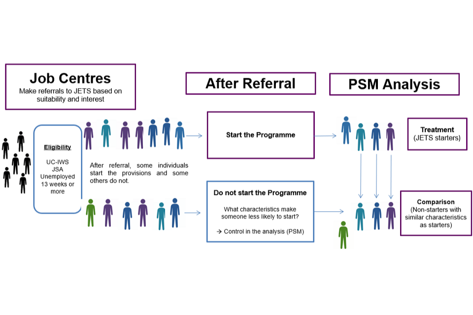
Figure 3.1 illustrates the process of referring claimants to JETS and the impact evaluation approach we followed in this report. Those individuals assessed as suitable and who started the provision after being referred form the treatment group. A comparison group with similar characteristics to those starting JETS is then created with Propensity Score Matching (PSM) using the sample of individuals assessed suitable, interested in participating, but that decided not to start after being referred to the programme.

3.3. PSM with administrative data

Our PSM analysis benefits from our capacity to construct a suitable comparison group to JETS participants exploiting rich administrative data. That is, we can match participants and non-participants on:

• a large array of relevant individual characteristics and
• repeated measures of key variables

For instance, we can construct a comprehensive historical profile of attachment to the labour market and barriers to employment. Key measures include employment and benefit histories, labour market transitions, occupation, earnings, care responsibilities, and disabilities, among others. More information on the data and the sources can be found in Appendix A. Moreover, to the extent that individuals’ labour market histories correlate well with unobserved factors like motivation to find employment, achieving a successful balance on previous employment and benefit spells will also make the participant and comparison groups more similar on unobserved characteristics. More importantly, it will make the two groups more similar on both observed and unobserved factors linked to both the decision to participate in the programme and subsequent labour market outcomes. For instance, while Caliendo et al. (2014) show that unobserved characteristics like personality traits, attitudes, expectations, and job search behaviour play a significant role for selection into treatment and labour market outcomes, their effect on impact estimates are minimised in specifications that include rich and detailed labour market histories.

As set out above, we restricted the comparison pool to those individuals who had been referred but did not start – based on a belief that this group would be more similar to participants than those who did not get as far as being referred. As a check we also carried out a comparison based on a wider pool of non-referred eligible individuals, which supported our choice – this is set out in Appendix E.

3.4. Sample selection

A total of 315,631 unique individuals were referred to JETS between Oct-20 and Nov-21. Our treatment group (n=203,339) is composed of those who were referred to the scheme before Dec-21 and started it. It excludes those who had more than one start (377 individuals removed, 0.2%)^{[footnote 9]}, those for whom we hold no information on individual characteristics in our systems (9 individuals) and those that show as registered with a Jobcentre Plus located in Scotland (250 individuals, 0.1%). See Figure 3.2 below.

Figure 3.2: Analysis sample selection

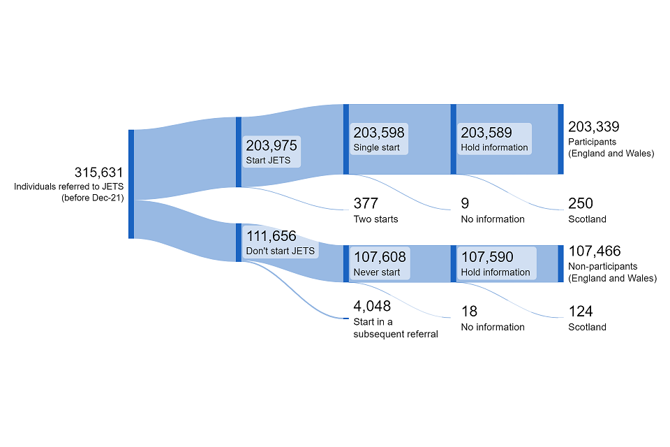
Figure 3.2 illustrates how individuals referred to JETS before December 2021 are defined as participants and non-participants in the analysis sample. Those individuals referred and that start the scheme are defined as participants. Those individuals who are referred but do not start the scheme are defined as non-participants.

Our main comparison pool (n=107,466) is derived from those referred to the scheme between Oct-20 and Nov-21 who did not start it, excluding those who start in a subsequent referral (4,048, 3.6%), those for whom we hold no information on individual characteristics (18 individuals) and that show as registered with a Jobcentre Plus located in Scotland (124 individuals, 0.1%).^{[footnote 10]},^{[footnote 11]}

Our alternative comparison sample (n= 278,978) is randomly selected among those who were claiming UC-IWS at the time JETS was taking referrals and were never referred to the scheme.^{[footnote 12]} More information on the selection of this group can be found in Appendix E.

Sample selection

Treatment group: Referred to JETS and started the provision

Comparison group:

• Referred to JETS and not started the provision
• UC-IWS wider comparison group (not referred to the provision)

3.5 Assessing labour market outcomes

This report inspects the impact JETS had on employment, earnings, and unemployment related benefits (out-of-work or low-income benefits) for up to three years after programme start. We present impact estimates for:

• The All cohort (main sample): Those referred to the programme from October 2020 to November 2021 (allows tracking outcomes for two years after programme start).
• The Early cohort: Referred to the programme in October and November 2020 (allows tracking outcomes for three years).

We perform the main analysis on the larger group of JETS referrals (All cohort) as it provides impact estimates that are more representative of the population that received support from JETS. We estimate programme effects for an early group of referrals (Early Cohort) to infer future impact estimates (three years after starting the provision). The All cohort sample accounts for two thirds (67%) of all programme referrals (9% in the case of the Early Cohort).

See Figure 3.3 for more information on the timing of the JETS scheme and the evolution of the labour market. Referrals to JETS started after a large drop in payrolled employment and a steep increase of UC claimants with a searching for work conditionality. When referrals ended, the level of employment was back to what it would have been had the pre-Covid trend continued. Similarly, the number of individuals on UC with searching for work requirements had reduced considerably after the initial spike.

Figure 3.3: Timing of JETS and the labour market environment

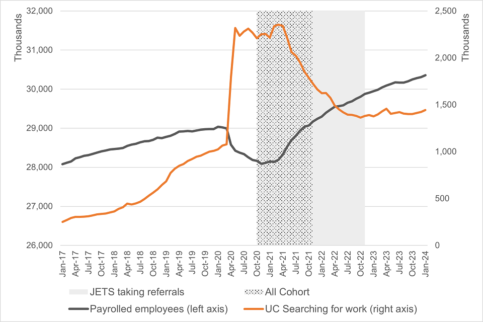
Figure 3.3 shows the evolution in payrolled employment and the number of individuals receiving Universal Credit with searching for work conditionality between January 2017 and January 2024 in the UK. The figure shows referrals to JETS started after a large drop in payrolled employment and a steep increase in the number of UC claimants with searching for work requirements. When referrals ended (September 2022), the level of employment had returned to what it would have been had the pre-Covid trend continued. Similarly, the number of individuals on UC with searching for work requirements had reduced considerably after the initial spike.

Source: Pay As You Earn Real Time Information from HM Revenue and Customs and Department for Work and Pensions (DWP Stat-Xplore).

To assess the impact of JETS at helping claimants back into employment we construct employment measures using payment data collected by HM Revenue and Customs (HMRC) through the Real Time Information (RTI) system. RTI is the reporting system for income taxed via Pay-As-You-Earn (PAYE). Through RTI we capture both earnings and time spent in payrolled employment.

We also measure out-of-work or low-income benefit receipt status and spells using different benefit datasets managed by the Department for Work and Pensions (DWP). Out-of-work or low-income benefits include Universal Credit with searching for work requirements (UC-IWS), Jobseeker’s Allowance (JSA), Income Support (IS), Employment and Support Allowance (ESA), Incapacity Benefit (IB), Severe Disablement Allowance (SDA), and Training Allowance (TA).

Moreover, we further disaggregate benefit receipt status by splitting out-of-work benefits between those who have requirements to search for work (looking for work benefits) and those who do not (other out-of-work/low-income benefits). Appendix A provides more details on the data and its sources.

We also assess the role of JETS at preventing individuals from moving into a status of neither in employment nor on benefits – ‘Other’ category. While the ‘Other’ category might include individuals moving into self-employment and not claiming benefits, or still looking for work but with no access to benefits, among others, it most likely captures – in large part –  individuals whom by choice or otherwise, temporarily or permanently, left the labour market.

List of employment outcomes:

Payrolled employment:

• Whether in employment ^{[footnote 13]}
• Days spent in employment
• Earnings from employment

Out-of-work benefits:

• Whether on benefits
• Days spent on benefits

Further divided by:

• Looking for work benefits (unemployment-related benefits with searching for work requirements)
• Other out-of-work/low-income benefits (unemployment-related benefits with no searching for work requirements)

Other (not in employment nor benefits):

• Whether not in employment nor benefits
• Days spent not in employment nor benefits

4. Matching quality

4.1. Common support

The success of a PSM analysis is in large part assessed by how well participants can be matched to non-participants based on individual and other relevant characteristics. The first consideration is the degree of similarity in propensity scores (the probability to participate in JETS) between those who start the provision and those who do not. Ideally, we would like to observe a similar distribution of the propensity scores between participants and non-participants and a high level of overlap.^{[footnote 14]}

We estimate the propensity score to participate in JETS using a logit model that includes the following covariates:

• Labour market history: employment and benefit receipt in the 2 years prior to referral to JETS.^{[footnote 15]} Labour market transitions between employment-unemployment-inactivity in the 3 months prior to referral. Income trajectories (from payrolled employment) in the 2 years leading to the referral using the inverse hyperbolic sine (IHS) transformation of earnings^{[footnote 16]}
• History of previous referrals to other specialised employment support programmes
• Personal characteristics including age, sex, family circumstances (living with a partner and/or with dependent children), ethnicity, socio-economic occupation, and the experience of disabilities
• Local labour market environment (unemployment rate, vacancy rate, and intensive work search rate at the time of referral)
• Jobcentre Plus Geography identifiers and date of referral

A more detailed list of the matching variables used can be found in Appendix F.

The variables described above are thought to potentially influence both employment and benefit outcomes as well as the decision to participate in JETS. Figure 4.1 displays the estimated propensity scores. While on average JETS participants have higher propensity scores than non‑participants – with a median propensity score of 0.69 and 0.61, respectively – the two distributions are fairly similar and there exists good common support when applying commonly used bandwidths (only 1 participant cannot be matched to non-participants).^{[footnote 17]}

Figure 4.1: Common support – Main sample

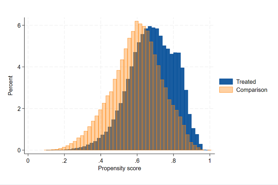
Figure 4.1 displays the estimated propensity scores for the treatment and the comparison group in the main sample. The two distributions are fairly similar and there exists good common support ranging approximately between 0.1 and 1.

4.2. Balance after matching

The main estimates are derived when matching each participant to 4 non-participants on their propensity score using nearest neighbour matching with replacement and a calliper width of 0.01.^{[footnote 18]}, ^{[footnote 19]}

Table 4.1 shows a summary of relevant statistics that are helpful at assessing the overall quality of the matching algorithm at creating a comparison group. After the matching, Rubin’s B and Rubin’s R are 5.8 and 1.0 respectively, well within the accepted thresholds for a balanced sample. The maximum % bias on the group of all covariates is 1.6, with the mean and median % bias of covariates set at 0.3%.^{[footnote 20]}

Table 4.1: Summary statistics of the matching exercise – Main sample

	Unmatched	Matched
Mean bias (%)	5.8	0.3
Median bias (%)	4.4	0.3
Max bias (%)	23.8	1.6
Rubin B	62.1	5.9
Rubin R	1.0	1.0

Figure 4.2 displays the standardised mean differences (SMDs) of a key set of covariates between the treatment and the comparison group before and after the matching (expressed as a percentage). Orange circles display SMDs before the matching exercise. Blue circles depict SMDs in the matched sample. The black dashed vertical lines represent a common acceptable range in covariate differences (between -3% and 3%). After the matching, differences in covariates are close to 0 (ranging from -1.12% to 1.59%).^{[footnote 21]}

Figure 4.2: Standardised mean difference (%) – Main sample

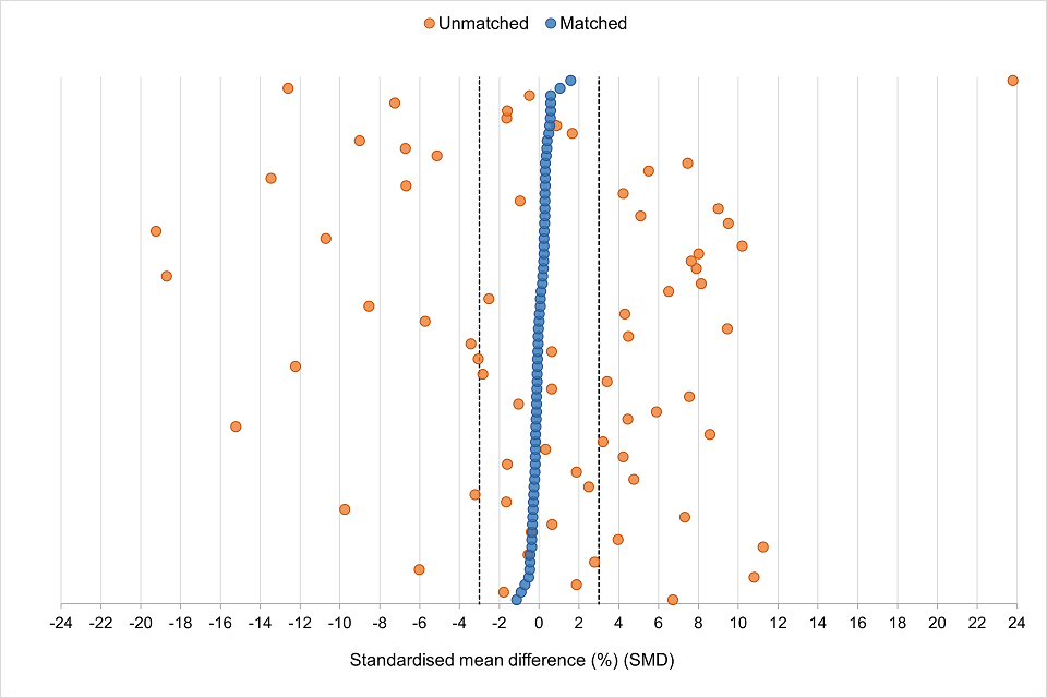
Table 4.2 displays a descriptive summary of a selection of key covariates for both the unmatched and matched samples and shows the high degree of success of the PSM at reducing initial differences in characteristics that are likely linked to performance in the labour market. For instance, males represent 58% of participants and 60% of non-participants in the unmatched sample. After matching, males account for 58% of individuals in both the participant and comparison groups – a reduction of the initial difference of 98.9% (from a standardised mean difference or bias of -3.4% to 0.0%). Similarly, a t-test of mean differences shows there are no statistically significant differences in the proportion of males in the treatment and comparison group after the matching (p-value of 0.90).

The good balance observed using rich administrative data, together with the referral process to the scheme– which filters individuals based on programme’s suitability and initial interest in employment support – improves the confidence in the validity of the impact estimates presented in the next section.

A more detailed summary of matching variables balance can be found in Appendix G.

Table 4.2: Balancing statistics – Main sample

Variable	Sample	Treatment	Comparison	% Bias	Reduction	t-stat	p-value
Male	Unmatched	0.58	0.60	-3.4	–	-9.05	0.00
Male	Matched	0.58	0.58	0.0	98.9%	-0.12	0.90
Age	Unmatched	38.2	37.3	7.3	–	19.39	0.00
Age	Matched	38.2	38.2	-0.3	95.6%	-1.02	0.31
Age group: 18-24	Unmatched	0.11	0.13	-6.7	–	-17.98	0.00
Age group: 18-24	Matched	0.11	0.11	0.4	93.9%	1.35	0.18
Age group: 25-49	Unmatched	0.67	0.66	0.6	–	1.70	0.09
Age group: 25-49	Matched	0.67	0.67	-0.1	85.0%	-0.31	0.76
Age group: 50+	Unmatched	0.22	0.20	4.8	–	12.59	0.00
Age group: 50+	Matched	0.22	0.22	-0.2	95.4%	-0.69	0.49
Disabled	Unmatched	0.15	0.14	2.8	–	7.38	0.00
Disabled	Matched	0.15	0.15	-0.4	83.9%	-1.41	0.16
Single parent	Unmatched	0.11	0.09	4.2	–	11.11	0.00
Single parent	Matched	0.11	0.11	0.3	92.7%	0.96	0.34
SOC: Elementary Occupations	Unmatched	0.16	0.16	0.6	–	1.69	0.09
SOC: Elementary Occupations	Matched	0.16	0.16	-0.06	90.5%	-0.19	0.85
SOC: Sales and Customer Service	Unmatched	0.13	0.11	3.42	–	9.02	0.00
SOC: Sales and Customer Service	Matched	0.13	0.13	-0.09	97.4%	-0.27	0.78
SOC: Administrative and Secretarial	Unmatched	0.06	0.05	4.46	–	11.68	0.00
SOC: Administrative and Secretarial	Matched	0.06	0.06	-0.14	96.8%	-0.44	0.66
SOC: Missing	Unmatched	0.45	0.48	-6.68	–	-17.73	0.00
SOC: Missing	Matched	0.45	0.45	0.31	95.3%	0.99	0.32
Referred to Work Programme	Unmatched	0.23	0.19	9.5	–	24.95	0.00
Referred to Work Programme	Matched	0.23	0.23	0.3	96.9%	0.90	0.37
Referred to other CEP	Unmatched	0.16	0.09	23.8	–	60.63	0.00
Referred to other CEP	Matched	0.16	0.16	1.6	93.3%	4.53	0.00
In employment 3 months pre-referral	Unmatched	0.09	0.13	-9.8	–	-26.36	0.00
In employment 3 months pre-referral	Matched	0.09	0.10	-0.3	96.9%	-1.02
In employment 12 months pre-referral	Unmatched	0.31	0.31	0.7	–	1.73	0.08
In employment 12 months pre-referral	Matched	0.31	0.31	-0.3	49.4%	-1.05	0.29
On OoW benefits 3 months pre-referral	Unmatched	0.93	0.91	7.5	–	20.37	0.00
On OoW benefits 3 months pre-referral	Matched	0.93	0.93	-0.1	98.5%	-0.39	0.70
On OoW benefits 12 months pre-referral	Unmatched	0.31	0.31	0.7	–	1.73	0.08
On OoW benefits 12 months pre-referral	Matched	0.31	0.31	-0.3	49.4%	-1.05	0.29
On OoW benefits 24 months pre-referral	Unmatched	0.33	0.29	9.0	–	23.77	0.00
On OoW benefits 24 months pre-referral	Matched	0.33	0.33	0.3	96.7%	0.93	0.35
Days in employment over 24 months pre-referral	Unmatched	199.0	200.3	-0.5	–	-1.44	0.15
Days in employment over 24 months pre-referral	Matched	199.0	200.0	-0.4	17.9%	-1.44	0.15
Days on OoW benefits over 24 months pre-referral	Unmatched	419.4	395.4	10.2	–	26.99	0.00
Days on OoW benefits over 24 months pre-referral	Matched	419.4	418.8	0.3	97.5%	0.80	0.43
Days on an active benefit over 24 months pre-referral	Unmatched	380.3	361.9	8.0	–	21.15	0.00
Days on an active benefit over 24 months pre-referral	Matched	380.3	379.7	0.2	96.9%	0.77	0.44
Days on an inactive benefit over 24 months pre-referral	Unmatched	39.12	33.58	4.3	–	11.28	0.00
Days on an inactive benefit over 24 months pre-referral	Matched	39.12	39.09	0.0	99.5%	0.07	0.95
Cumulative transformed earnings over 24 months pre-referral	Unmatched	5.61	5.52	1.9	–	5.00	0.00
Cumulative transformed earnings over 24 months pre-referral	Matched	5.61	5.65	-0.7	63.1%	-2.21	0.03

 5. Programme Impacts

 5.1. Main effects

Results show that JETS had a positive impact on a wide range of labour market outcomes. Those receiving support from the scheme spent more time in payrolled employment – therefore securing higher earnings –, were less dependent on out-of-work or low‑income benefits, and less likely to leave the labour market.

The solid blue line in Figure 5.1 shows the evolution in the proportion of JETS participants in payrolled employment before and after starting the scheme. The grey dashed line shows the proportion in employment among those referred to the scheme that did not start the programme, and the orange line displays the proportion in employment among our constructed comparison group using PSM (the counterfactual).

After 2 years of being referred to JETS, 44.8% of participants were in payrolled employment, compared to about 36% in the matched comparison sample. This difference in employment levels across groups can be attributed – subject to satisfying the CIA – to the programme and it is displayed in Figure 5.2.

Figure 5.2 shows there were no differences in payrolled employment levels between participants and matched non-participants over the 2 years prior to being referred to the programme (vertical dashed line at the 0-axis). Since then and after a short ‘lock‑in’ effect period of lower employment, those who received support from the scheme were more likely to be in payrolled employment than those who did not (8.2 pp higher employment at year 1 and 8.8 pp higher employment at year 2).^{[footnote 22]} The light blue area represents the 95% confidence interval of the point estimates.

Figure 5.1: Proportion in payrolled employment by group – Main sample

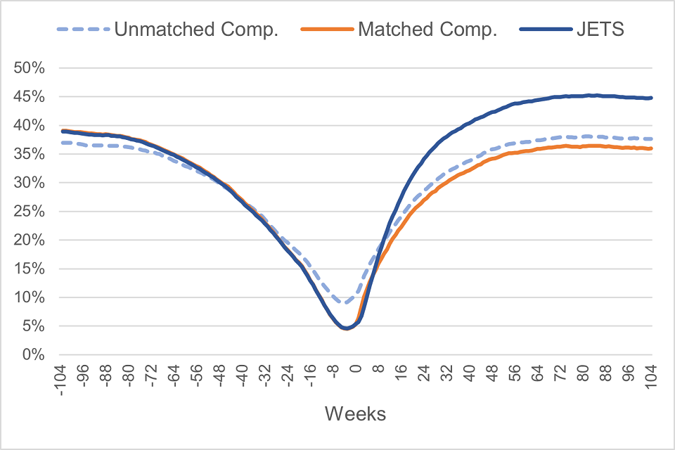
Figure 5.1 shows there was a similar employment level between participants and matched non-participants over the 2 years prior to being referred to the programme. After referral, those who received support from the scheme were more likely to be in payrolled employment than those who did not (44.8% versus 36.0%, respectively, at year 2).

Figure 5.2: Percentage point difference in payrolled employment – Main sample

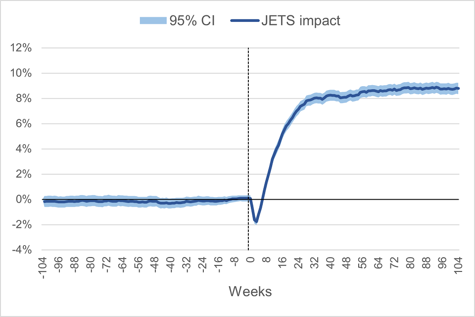
Figure 5.3 and Figure 5.4 show the evolution on out-of-work or low-income benefit receipt between participants and the comparison group. Similarly, while there are no differences on benefit receipt between groups before programme referral, those who started JETS were 3 pp less likely to be claiming an unemployment related benefit two years later.

Figure 5.3: Proportion on out-of-work or low-income benefits – Main sample

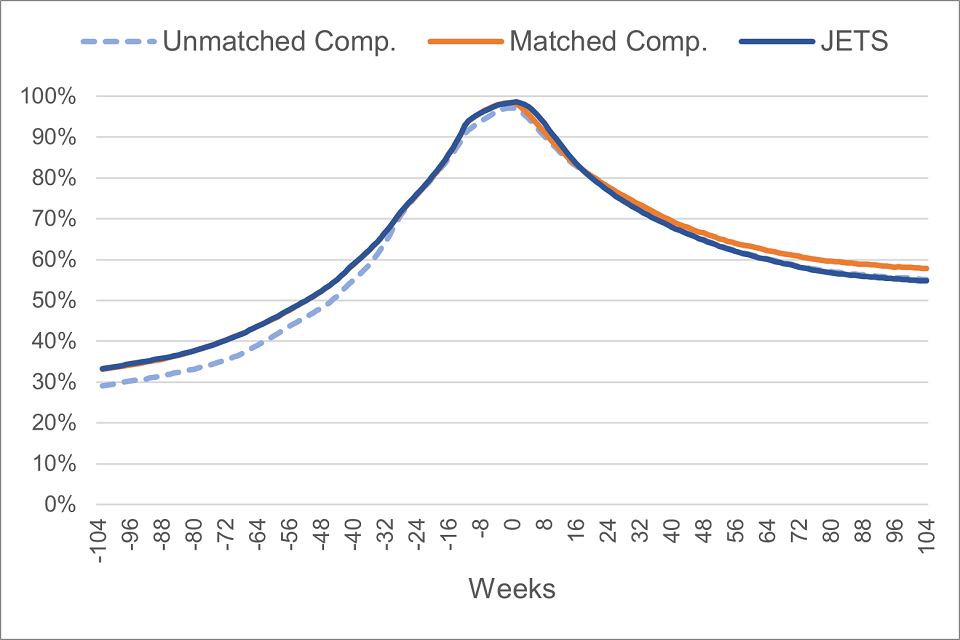
Figure 5.3 shows there was a similar proportion of individuals in out-of-work or low income benefits between participants and matched non-participants over the 2 years prior to being referred to the programme. After referral, those who received support from the scheme were less likely to be in out-of-work or low income benefits than those who did not (54.8% versus 57.8%, respectively, at year 2).

Figure 5.4: Percentage point difference on out-of-work or low-income benefits – Main sample

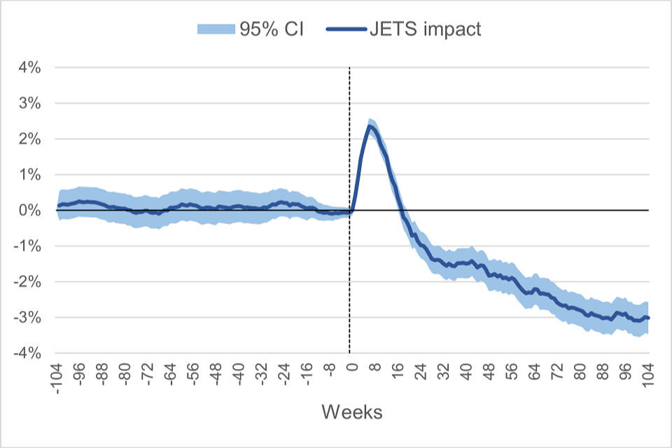
Figure 5.4 shows there were no differences in out-of-work or low income benefit receipt between participants and matched non-participants over the 2 years prior to being referred to the programme. Since then and after a short ‘lock in’ effect period of higher benefit receipt, those who received support from the scheme were less likely to be in out-of-work or low income benefits than those who did not (1.8 pp less likely at year 1 and 3.0 pp less likely at year 2). The light blue area represents the 95% confidence interval of the point estimates.

The cumulative effects from participating in JETS are shown in Table 5.1. On average and after two years from having started the scheme, those on JETS spent 53 additional days (7.2 pp) in payrolled employment and 11 fewer days (1.6 pp) on out-of-work or low‑income benefits. It is worth mentioning that because of the design of Universal Credit – where benefits are compatible with lower levels of income from employment – additional days in payrolled employment do not automatically translate to fewer days on benefits. On average, the increased attachment to the labour market resulted in about £2,550 additional earnings, with participants 5.8 percentage points (pp) more likely to have earned at least £20,000 since joining the scheme (see Appendix Figure B.5 on the evolution of additional cumulative earnings).

Similarly, while over 42% of the comparison group was unable to find employment during the period of analysis (remained jobless), this percentage was 32% among the sample of participants (10 pp lower).

Table 5.1: JETS impact over 2 years – Main sample

Payrolled employment	Treatment	Comparison	Impact	[95% CI]
Days	277	225	53	[50 , 55 ]
Level (pp)	38.1	30.9	7.2	[6.9 , 7.6]

Earnings	Treatment	Comparison	Impact	[95% CI]
Cumulative earnings (£)	12,785	10,236	2,549	[2,399 , 2,699]
Achieved £1K (pp)	62.5	52.2	10.3	[9.8 , 10.7]
Achieved £20K (pp)	25.8	20.1	5.8	[5.4 , 6.1]
Jobless	31.9	42.1	-10.2	[-10.7 , -9.8]

Out-of-work (OoW) benefits	Treatment	Comparison	Impact	[95% CI]
Days	492	503	-11	[-14 , -9]
Level (pp)	67.5	69.1	-1.6	[-1.9 , -1.2]
Looking for work benefit: Days	439	429	10	[8 , 12]
Looking for work benefit: Level (pp)	60.3	58.9	1.4	[1.1 , 1.7]
Other OoW benefit: Days	53	74	-21	[-23 , -20]
Other OoW benefit: Level (pp)	7.2	10.2	-2.9	[-3.1 , -2.7]

Other category	Treatment	Comparison	Impact	[95% CI]
Days	74	95	-21	[-23 , -19]
Level (pp)	10.1	13.0	-2.9	[-3.1 , -2.7]

Table 5.2 shows the proportion of individuals in each of the labour market categories assessed by treatment status at the end of each year since being referred to the programme. After 1 year, 43.0% of JETS participants were employed (compared to 34.8% in the comparison group). The difference in payrolled employment between the two groups grows to 8.8 pp at year 2 (44.8% versus 36.0%).

Breaking down the type of benefit received by conditionality, Table 5.2 shows JETS reduced the likelihood of jobseekers moving to other out-of-work/low-income benefits (with no searching for work requirements) and was able to retain more claimants in the looking for work benefit – closer to the labour market. After 2 years, those supported by the JETS scheme spent 10 more days on a looking for work benefit and 21 fewer days on other out-of-work/low-income benefits (see Table 5.1).

Similarly, JETS reduced the proportion of individuals in the ‘Other’ category (not in employment nor on an out-of-work or low-income benefit), preventing an increased detachment from the labour market. As a result, participants spent, on average, 21 days fewer in this category.

Table 5.2: Impact at of each follow-up year - Main sample

Payrolled Employment (pp)	Baseline	Year 1	Year 2
Treatment	5.3	43.0	44.8
Comparison	5.2	34.8	36.0
Impact [95% CI]	–	8.2 [7.8 , 8.6]	8.8 [8.4 , 9.2]

Out-of-Work (OoW) benefits (pp)	Baseline	Year 1	Year 2
Treatment	98.6	63.3	54.8
Comparison	98.6	65.1	57.8
Impact [95% CI]	–	-1.8 [-2.3 , -1.4]	-3.0 [-3.5 , -2.6]
Looking for work benefit (pp): Treatment	97.1	56.5	40.9
Looking for work benefit (pp): Comparison	97.0	54.9	39.9
Looking for work benefit (pp): Impact [95% CI]	–	1.6 [1.2 , 2.1]	1.1 [0.6 , 1.5]
Other OoW benefit (pp): Treatment	1.5	6.8	13.9
Other OoW benefit (pp): Comparison	1.5	10.3	17.9
Other OoW benefit (pp): Impact [95% CI]	–	-3.4 [-3.7 , -3.2]	-4.1 [-4.4 , -3.7]

Other category (pp)	Baseline	Year 1	Year 2
Treatment	1.1	11.1	14.9
Comparison	1.1	14.3	18.3
Impact [95% CI]	–	-3.2 [-3.5 , -2.9]	-3.4 [-3.7 , -3.0]

Additional figures on the evolution of labour market outcomes and programme effects can be found in Appendix B.

5.2. Long-term effects: The Early Cohort

Evaluating the impact JETS had on an early group of participants (those referred in Oct/Nov 2020) allows to make inferences on the continuation of overall programme effects beyond the 2 years observed for the main sample (referred up until Nov 2021). To make inferences about continuing programme effects using the Early cohort we need to assess:

1. How similar/dissimilar are programme effects between the Early and the All Cohort (main sample) in the first 2 years after starting JETS.
2. Whether programme effects for the Early Cohort increase, decrease, or stabilise over time (between year 2 and 3).

Figures 5.5 and 5.6 show a similar pattern of increased payrolled employment and reduced benefit receipt between the Early and the All Cohort. More importantly, estimates show sustained impact effects between year 2 and 3 after programme start (with no sign of impact decay).

Figure 5.5: Percentage point difference in payrolled employment – All (main sample) vs Early Cohort

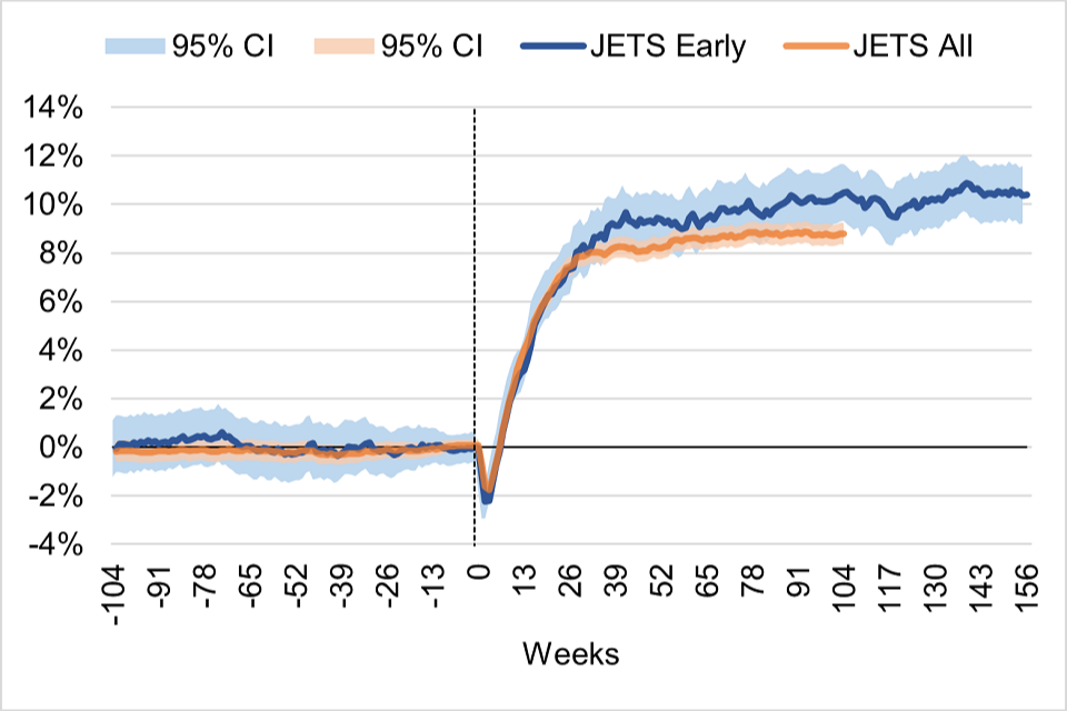
Figure 5.6: Percentage point difference on out-of-work or low-income benefits – All (main sample) vs Early Cohort

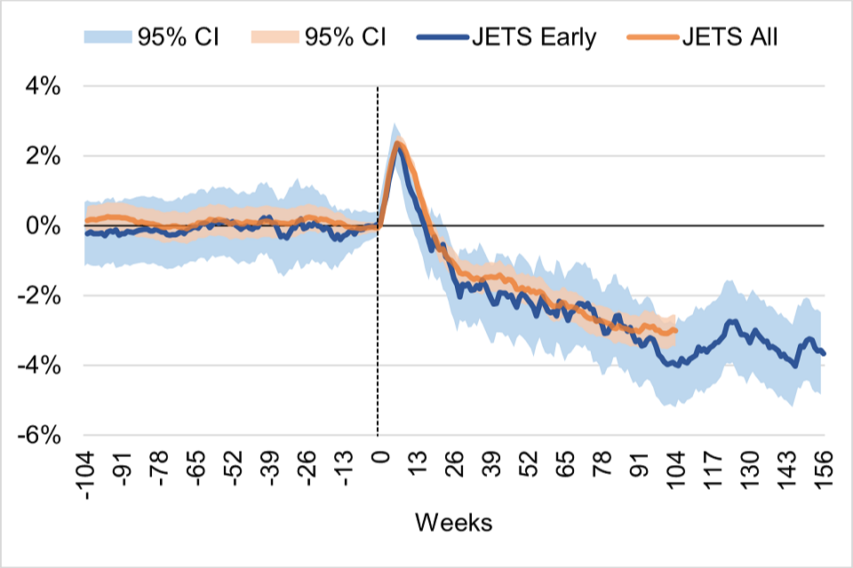
If anything, employment effects seem slightly larger among early participants compared to the wider group of referrals – 0.7 pp higher impact on additional days in payrolled employment and 0.2 pp higher impact on reducing the number of days in receipt of out-of-work or low-income benefits over the first 2 years since programme start (see Table 5.3).

Table 5.3: JETS impact over 2 years – All Cohort (main sample) vs Early Cohort

Payrolled employment	Early Cohort, Impact [95% CI]	All Cohort, Impact [95% CI]
Days	58 [52 , 64]	53 [50 , 55]
Level (pp)	7.9 [7.1 , 8.8]	7.2 [6.9 , 7.6]

Earnings	Early Cohort, Impact [95% CI]	All Cohort, Impact [95% CI]
Cumulative earnings (£)	3,014 [2,613 , 3,415]	2,549 [2,399 , 2,699]
Achieved £1K (pp)	11.2 [10.0 , 12.3]	10.3 [9.8 , 10.7]
Achieved £20K (pp)	7.1 [6.1 , 8.1]	5.8 [5.4 , 6.1]
Jobless	-11.0 [-12.1 , -9.9]	-10.2 [-10.7 , -9.8]

Out-of-work (OoW) benefits	Early Cohort, Impact [95% CI]	All Cohort, Impact [95% CI]
Days	-13 [-19 , -8]	-11 [-14 , -9]
Level (pp)	-1.8 [-2.6 , -1.0]	-1.6 [-1.9 , -1.2]
Looking for work benefit: Days	4 [-2 , 10]	10 [8 , 12]
Looking for work benefit: Level (pp)	0.5 [-0.2 , 1.3]	1.4 [1.1 , 1.7]
Other OoW benefit: Days	-17 [-21 , -14]	-21 [-23 , -20]
Other OoW benefit: Level (pp)	-2.4 [-2.8 , -1.9]	-2.9 [-3.1 , -2.7]

Other category	Early Cohort, Impact [95% CI]	All Cohort, Impact [95% CI]
Days	-24 [-28 , -20]	-21 [-23 , -19]
Level (pp)	-3.3 [-3.9 , -2.7]	-2.9 [-3.1 , -2.7]

The reason impact estimates might have been slightly higher among those starting JETS during its initial stages is likely related to the circumstances of the period. During the initial JETS rollout in Autumn 2020 there was little employment support from Jobcentre Plus, many of the interactions were digital, and not many people were going on other programmes. As a result, the comparison group at the time may have experienced lower support than usually available during normal conditions.^{[footnote 23]}

Additional figures comparing other labour market outcomes between the Early and the All cohort can be found in Appendix B.

Moreover, estimates show that at the 3-year mark since programme start JETS participants from the Early Cohort had a 10.4 pp higher payrolled employment rate, 3.7 pp lower rate of out-of-work/low-income benefit receipt, and had accumulated over £5,300 more from earnings than those who did not start JETS. See Appendix C for more detailed results on the analysis of programme effects for the Early Cohort.

As a result, we anticipate JETS to continue generating positive effects among participants beyond the initial 2 years observed. We use the findings from this exercise to extrapolate programme effects beyond the 2-year tracking period when evaluating the cost-effectiveness of the scheme in the Cost Benefit Analysis section of the report.

5.3. Sensitivity of impact estimates

To alternative model specifications

We assess the sensitivity of the main impact estimates to different model specifications. Details of the analysis can be found in Appendix D. All in all, results show impact estimates are robust to alternative model specifications and the use of alternative PSM parameters.

To an alternative comparison sample

As explained previously, our main estimates of programme effects compare the labour market outcomes of those who started JETS with a comparison group created from those who did not start the programme after being referred to it. As a sensitivity check, we estimate programme effects by comparing the outcome of participants with a comparison group created from a sample of individuals that were claiming UC-IWS but were never referred to the scheme. Details of the analysis can be found in Appendix E.

The analysis shows that those who were never referred to the scheme are less similar to participants than those who were referred but did not start. Results show larger impact effects when using the non-referred sample (4.9 pp higher payrolled employment rate at year 2). This difference we believe is attributable to there being unobserved variables which affect the referral process – supported by a further PSM analysis which showed a difference of 5 pp in the payrolled employment rate at year 2 between those who were referred but did not start and the non-referred group, even after controlling for all the observed factors.

5.4. Contemporaneous employment support

As mentioned earlier, JETS co-existed with other contracted employment schemes. This means that both participants and non-participants could have started alternative and/or additional employment support during the period of observation.

While impact estimates capture the effect of participating in JETS, this effect is influenced by the decision among individuals in our sample to start other provisions. For instance, those who were referred to JETS but did not start the provision could have done so to start another programme. This would result in an underestimation of JETS ability at creating additional employment. Similarly, those who started JETS and were unsuccessful at finding employment could have benefited from additional employment support following JETS. This would overestimate JETS ability (in isolation) of increasing employment prospects among participants.

Figure 5.7 shows that 29.3% of JETS participants and 27.1% of matched non‑participants (the comparison group) started other employment support in the 2 years following referral to JETS. These figures are primarily driven by the share of individuals starting Restart across groups (26.6% vs 23.1% in the participant and comparison group, respectively). On the other hand, a higher proportion of individuals in the comparison group started the WHP (1.4 pp higher participation relative to the participant group). The Other smaller combined category comprises participation in the IPES, ESF, JFS, and NEA Phase 2 programmes (described in Section 1.5 of the report).^{[footnote 24]}

Figure 5.7: Starts in other contracted provisions within 2 years following referral to JETS

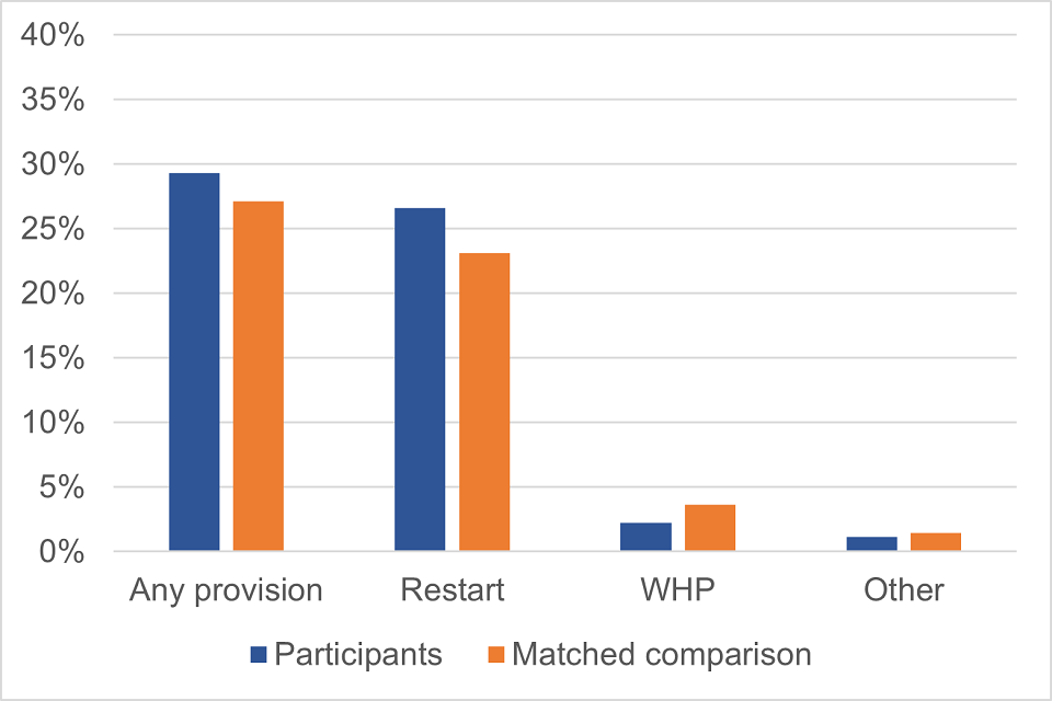
Ultimately, the effect of participation in other provisions on the JETS impact estimates will depend on how successful these other programmes are at increasing employment among participants. Given the relatively small difference in participation rates in other programmes across JETS participants and the comparison group (2.2 pp difference), we expect a marginal effect of contemporaneous programmes on the JETS impact estimates.

5.5. Programme effects by population groups

This section provides a closer assessment to the effect that participation in JETS had on different population groups. More specifically, Figure 5.8 displays the additionality in payrolled employment over the 2 years following referral split by sex, age, time on out-of-work benefits and regions.^{[footnote 25]}

Results show a higher effect from programme participation among females than males (8.2 pp versus 6.4 pp in additional payrolled employment, statistically and significantly different at the 1% level). The analysis of programme effects by age group shows a clear gradient, with JETS increasing the payrolled employment rate by 9.4 pp among those aged 18 to 24, by 7.2 pp among the 25 to 49 age group, and by 5.6 pp among those aged 50 or more (all differences between groups statistically significant at the 1% level).

Assessing employment effects by the duration of the most recent out-of-work benefit spell, Figure 5.8 shows the highest impact among those who were between 7 to 12 consecutive months on out-of-work benefits at the point of referral (8.0 pp). On the other hand, the lowest impact is estimated for those with a benefit spell of 24 months or higher.^{[footnote 26]}

The analysis shows that JETS had a positive impact in all regions. The highest impact was in the North West (10.8 pp) and the lowest impact was in Central England (6.0 pp). The difference in impact between these regions and the aggregate effect for England and Wales is statistically significant at the 1% level. Except for Southern England (with an estimated employment additionality of 8.0 pp – statistically and significantly different to the overall effect at the 10% level) participants across all the other regions experienced similar positive employment effects. There are many factors that might affect these regional findings, including differences in the characteristics of participants and non-participants across regions, varying levels of alternative employment support, and/or differences in the evolution of local labour markets, among others.

Figure 5.8: Impact effects by sub-population groups: Proportion in payrolled employment over 2 years after programme start

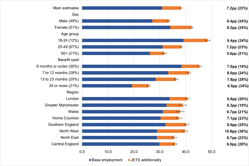
Figure 5.8 shows the percentage point additionality in payrolled employment over 2 years from participating in JETS and for different sub-population groups. By sex: males (6.4 pp), females (8.2 pp); by age groups: 18 to 24 (9.4 pp), 25 to 49 (7.2 pp), 50+ (5.6 pp); by the duration of the most recent benefit spell: 6 months or under (7.0 pp), 7 to 12 months (8.0 pp), 13 to 23 months (7.8 pp), 24 or more (6.5 pp); by region: London (6.9 pp), Greater Manchester (6.3 pp), Wales (6.7 pp), Home Counties (7.1 pp), Southern England (8.0 pp), North West (10.8 pp), North East (6.7 pp), Central England (6.0 pp).

Note: Estimates are derived by conducting a separate PSM analysis for each subgroup. Base employment shows the level of employment of the matched comparison group. JETS additionality shows the percentage point difference between the level of employment among JETS participants and the matched comparison group. The percentage increase (%) in the employment level is displayed in brackets.

The findings from this exercise would suggest that the type of employment support offered by JETS is particularly beneficial among young claimants, who might be relatively new to the labour market and/or might have had less time to develop relevant skills. If we consider that spells of unemployment early in life can have long-lasting consequences, intervening in this group would seem particularly advantageous.

Similarly, females seem to have disproportionately benefited more from the support offered by JETS than males. This could signal increased barriers to employment experienced among this group (for instance, due to a reduced network, information, or relevant contacts in the job search; or due to a higher level of caring responsibilities, among others).

An assessment of programme effects by the duration of the most recent out-of-work benefit spell shows that, while the payrolled employment rate increased by 6.5 pp among the group with the longest out-of-work benefit spell (the lowest of all groups) this represents a 34% increase (from 19.3 pp to 25.8 pp), the highest of all benefit duration groups.

6. Cost Benefit Analysis

This section presents the Cost Benefit Analysis (CBA) of JETS (Job Entry Targeted Support), where the benefits derived from increased employment among participants are compared against the cost of the scheme.

6.1. CBA Methodology

We perform the analysis following the guidance set out in the Green Book – issued by HM Treasury on how to appraise policies, programmes, and projects – and using the DWP Social Cost Benefit Analysis (SCBA) framework as set out by Fujiwara (2010). This is a recognised piece of supplementary guidance to the Green Book which has been scrutinised and approved for use within DWP – other departments each have their own standard methodology. This framework is consistent with previous DWP impact evaluations and with the development of departmental business cases.^{[footnote 27]} The following sections outline how this approach was applied to JETS, whose perspectives are being considered, which costs and benefits are included and the scale of these.

This framework, however, excludes a number of costs and benefits where it was not possible to obtain robust evidence, for example, the additional childcare costs incurred both by participants after entering employment and by the exchequer/DWP in the form of increased UC childcare allowance. Further details on the limitations of the adopted methodology are also discussed.

6.1.1. Perspectives under consideration

The costs and benefits are considered from the perspectives of:

• The JETS participant
• The Employer
• The Exchequer
• Society
• The Department for Work and Pensions (DWP)

The JETS participant perspective primarily considers the individual changes in wages and benefits received by those on the programme. The employer perspective considers the increase in economic output produced by employees and the increase in wages and national insurance contributions paid by the employer. In this CBA, the costs and benefits for the employer are always equal, as there are no employer subsidies or additional costs to the employer, meaning the benefit-cost ratio is always £1. The Exchequer – or government budget perspective – includes the benefits and costs accruing to the DWP in addition to other fiscal benefits like income tax receipts.

The society perspective represents the net impact from the other perspectives, with society representing an aggregate of all British citizens. When all perspectives are considered, some elements cancel out as they represent an equal benefit and cost from two different perspectives, such as wages (benefit for participants, cost for employers) and income tax (cost for participants, benefit for the exchequer).^{[footnote 28]}  

The DWP perspective considers reductions in benefits payments departmental operational costs, and the cost of running the programme. These form part of the costs and benefits for the exchequer, and so these perspectives are not mutually exclusive.

Different costs and benefits are considered for each of these perspectives, and cost benefit ratios can be calculated based on estimates of these. The cost benefit ratio represents the value returned for each £1 of cost incurred.

The main driver of the estimated costs and benefits are the impact results, i.e. the number of additional days spent in employment as a result of participation in the programme. As impact estimates carry some degree of uncertainty and programme benefits are subject to model assumptions, we further perform a sensitivity analysis on the value for money of the scheme.

6.1.2. Costs and benefits under consideration

The different monetised costs and benefits from the JETS scheme included in the CBA are detailed below and summarised in Table 6.1. The sign in Table 6.1 shows whether a specific element is considered a cost or a benefit (or has a null effect) depending on the perspective under consideration.

Table 6.1: Monetised costs and benefits of JETS

Impact	Participants	Employer	Exchequer	Society	DWP
Increase in economic output	0	+	0	+	0
Increase in wages	+	-	0	0	0
Programme costs	0	0	-	-	-
Reduction in operational costs	0	0	+	+	+
Reduction in benefits payments	-	0	+	0	+
Increase in taxes	-	-	+	0	0
Increase in travel costs	-	0	0	-	0
Redistributive costs and benefits	+	0	0	+	0
Monetised change in quality of life	+	0	0	+	0

Increase in output

This refers to the economic output produced by participants because of additional time spent in employment. This output represents a benefit to employers (who sell it) and society (who consume it). As we do not have information on the value of this output we make the simplifying assumptions below.

The labour market is assumed to be perfectly competitive. This implies that employers will hire workers up to the point where the value of an additional unit of output is equal to the associated marginal cost of production. The cost of production, and therefore the value of the output produced during additional spells in employment, is assumed to equal the commensurate gross wage payments and employers’ National Insurance contributions (NICs).

Increase in wages

This refers to the gross wages received by participants from additional time spent in employment. This is a benefit to the participants and an equal cost to their employers. From the society’s perspective there is no net benefit or cost, only a redistribution of resources. The increase in wages is calculated by taking the median weekly gross earnings among those participants in employment over the two-year tracking period (reported in the PAYE-RTI dataset). 

Programme costs

As set out in section 1, JETS operated under a Cost-plus model – paying 5% on top of the average cost of administering the programme per participant. The programme’s cost to the Exchequer is calculated at £823 per participant and is obtained through a weighted average of the service fee paid in the different areas (different providers) and the volumes each area supported.

Reduction in operational costs

Higher employment level and lower benefit receipt among JETS participants translates to a lower need of support from Jobcentre Plus advisers and other DWP employment programmes. This translates into operational savings which represent a benefit to the Exchequer and society – as economic resources can be reallocated to alternative uses.

Reduction in benefits

This refers to the net reduction in benefit entitlement and take-up that occurs when participants spend additional time in employment following participation on the JETS programme. This is treated as a transfer payment, representing a cost to participants but a benefit to the Exchequer – which means there is a null net cost or benefit to the Society (except via redistributive effects). Changes in benefit entitlement and take-up are estimated using the DWP Policy Simulation Model.^{[footnote 29]}

Increase in taxes

This refers to the increase in income tax, National Insurance and indirect tax revenue that occurs when participants spend additional time in employment as a result of participation in JETS. This represents a benefit to the Exchequer but a cost to participants and employers, which means there is no net cost or benefit to society (except via redistributive effects). Increases in tax revenue are estimated based on the increase in wages.

Increase in travel costs

This refers to the additional travel costs that are incurred by:

1. Participants: as a result of increased employment following participation in JETS.
2. The society: as the provision of additional travel services diverts economic resources from alternative uses. Moreover, there is an additional social cost from increased travelling due to, for instance, congestion or pollution.

Redistributive costs and benefits

This refers to the redistributive costs and benefits associated with monetary transfers between participants, employers, and the Exchequer. In line with the methodology prescribed in the HM Treasury Green Book (HM Treasury, 2022), participants, who have relatively low incomes, are assumed to attach a higher value to each additional pound than the average taxpayer (with a relatively higher income). This assumption is based on the economic principle of the diminishing marginal utility of income. In other words, individuals on lower incomes value an additional pound more than wealthier individuals. This implies that monetary transfers from the Exchequer to JETS participants represent a benefit to society as a whole.

Redistributive effects in this report are considered as part of the sensitivity analysis, not the main results. In line with the recommendations of Fujiwara (2010) – and as previously applied in the Universal Credit Business Case ^{[footnote 30]} – redistributive costs and benefits are estimated by applying a ‘welfare weight’ to monetary transfers made to and from programme participants. The welfare weight applied depends on the equivalised household income quintile of the participant before they start the programme, though most JETS participants will begin in the lowest income quintile. We know that participants are unemployed at the point of referral and that their median earnings from employment are 0. We also assume that participants don’t receive any non-employment income other than Universal Credit, and that partner earnings (where applicable) are 0.^{[footnote 31]}

Monetised change in quality of life

This captures the change in physical and mental wellbeing as a result of being in employment. These health outcomes are estimated using quality-adjusted life years (QALYs) – which combine longevity and level of health into a single measure – with 1 QALY representing a year in perfect health. The Department of Health estimates that a QALY has a monetised value of £70,000 in 2020/21 prices.^{[footnote 32]} Schuring et al. (2010) estimates the QALY gains associated with returning to employment at 0.068, which gives a monetised value of £4,760 (£70,000×0.068). The monetised QALY gain is attributed to the year in which an individual returns to employment. As JETS increased by 10.3 pp the proportion of individuals returning to employment (see Table 5.1 in section 5), we use that estimate to determine the QALY gain that can be attributed to the programme.^{[footnote 33]} For our example, this results in a monetised QALY gain of £490 per participant.

This represents a benefit to the participant and society and is included in the CBA only as part of the sensitivity analysis, not the main results.

6.1.3. Estimating the scale of the benefits under consideration

The scale of the costs and benefits of JETS depends on the magnitude and the duration of its impacts. In this case, the impacts are measured as the average number of additional days participants spent in employment relative to a similar group of non-participants. These additional days are derived in Section 5 of the report.

The main tracking period in this study covers two years from the point of referral, though we also estimate programme effects over three years for an early group of participants (Early cohort). Figure 5.5 shows sustained employment effects beyond year 2 for the Early cohort with no signs of impact decay. As a result, our baseline assumption when extrapolating programme effects is that employment additionality will follow the trend observed during the first 2 years of follow-up. As future effects from programme participation are uncertain, we also perform, as a sensitivity, a conservative extrapolation that assumes impact decays at an annualised rate of 25% between years 3 and 5 – after which employment additionality is assumed to be zero.^{[footnote 34]}

Figure 6.1: Actual and extrapolated cumulative additional days in employment

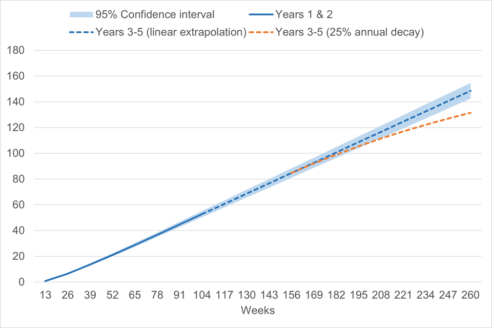
Figure 6.1 shows the evolution in the estimated and extrapolated cumulative additional days in employment from participating in JETS. At week 104 after referral, the cumulative additional days in employment are estimated at 52.7. A linear extrapolation of the observed effects shows 148.5 days of cumulative additional employment after 5 years. An extrapolation that assumes a 25% annualized decay of the impact shows 131.5 days of cumulative additional employment after 5 years. Confidence intervals at the 95% level are displayed for the estimated effects and for the linear extrapolation.

Table 6.2: Cumulative average additional days in employment in each year following referral to JETS

	Central	Lower bound (95% confidence interval)	Upper bound (95% confidence interval)	25% annualised decay
Year 1	21.1	19.9	22.2	21.1
Year 2	52.7	50.3	55.1	52.7
Year 3	84.7	81.0	88.3	84.7
Year 4	116.6	111.8	121.4	111.4
Year 5	148.5	142.5	154.6	131.5

Note: Additional days in employment at Year 1 and Year 2 are derived from Propensity Score Matching (PSM) impact estimates. Additional days in Years 3 to Year 5 are extrapolated using the impact estimates.

Table 6.3: In-year average additional days in employment in each year following referral to JETS

	Central	Lower bound (95% confidence interval)	Upper bound (95% confidence interval)	25% annualised decay
Year 1	21.1	19.9	22.2	21.1
Year 2	31.6	30.4	32.9	31.6
Year 3	31.9	30.7	33.2	31.9
Year 4	31.9	30.7	33.2	26.8
Year 5	31.9	30.7	33.2	20.1

Note: Additional days in employment at Year 1 and Year 2 are derived from Propensity Score Matching (PSM) impact estimates. Additional days in Years 3 to Year 5 are extrapolated using the impact estimates.

6.1.4. Limitations of this approach

The CBA estimates are subject to the same level of uncertainty as the impact estimates and the underlying model assumptions used to generate these. In addition, the assumptions underpinning the methodology of the CBA described earlier in this section directly affect the magnitude of the estimated results.

The CBA under this framework excludes some potentially significant costs and benefits where robust evidence is lacking. Any interpretation of the CBA estimates should consider these missing costs and benefits. These include:

• Additional leisure time foregone by participants.
• Non-pecuniary benefits associated with additional time in unsubsidised employment.
• The economic multiplier effect of the programme.
• Potential reduction in crime because of movement into employment.

See Fujiwara (2010) for a more detailed discussion of the non-monetised costs and benefits of employment programmes.

 6.2. Findings of cost benefit analysis

This section presents the estimated benefit-cost ratios (BCRs) of the JETS programme.

Baseline scenario estimates of the central impact with upper and lower bounds are presented first; at both the 2-year (materialised) and 5-year (expected) points. This is followed by a sensitivity analysis where varying options and assumptions are considered. BCRs are based on costs and benefits expressed in 2021/22 prices.

 6.2.1. Baseline estimates

Table 6.4 below lists the BCRs from each perspective using the central, lower, and upper bound estimates of additional days in employment.

Table 6.4: Baseline benefit-cost ratios

	Participant	DWP	Exchequer	Society
2 years (materialised): Central	£2.07	£0.73	£1.34	£2.53
2 years (materialised): Lower	£2.07	£0.70	£1.28	£2.42
2 years (materialised): Upper	£2.07	£0.77	£1.41	£2.63
2 years + 3 extrapolated (expected): Central	£2.06	£2.07	£3.68	£6.14
2 years + 3 extrapolated (expected): Lower	£2.06	£1.98	£3.53	£5.93
2 years + 3 extrapolated (expected): Upper	£2.06	£2.17	£3.83	£6.35

These results are presented graphically in Figure 6.2, with the error bars representing the BCRs under the lower and upper bound impact estimates. These are based on the uncertainty underpinning the estimation of the impact results, as well as the following:

• The value of output produced through participation in JETS is equal to the commensurate gross wage payments and employers’ national insurance contributions.
• JETS does not result in redistributive costs or benefits, substitution effects, or a social cost to the Exchequer (distribution and substitution effects are considered in the sensitivity analysis).

Figure 6.2: Baseline benefit-cost ratios

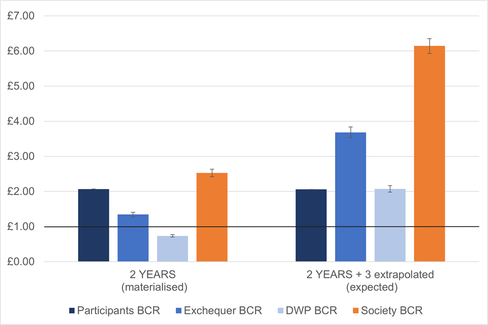
As noted previously, the reliability of the CBA is dependent on the robustness of the impact estimates as well as the assumptions used in the CBA modelling. Furthermore, the ‘expected’ view includes 3 years of extrapolated data – impact estimates are more uncertain the further into the future projections are made.

On average, JETS resulted in a net benefit for participants. For each £1 lost in the form of reduced benefits, higher taxes and NIC, and other costs such as increased travel, they gained £2.07 in increased wages and tax credits after 2 years. This figure remains almost the same when considering the expected 5 years of impacts (£2.06).^{[footnote 35]}

From the Exchequer perspective, each £1 spent in the programme returned £1.34 in the form of tax receipts, reduced benefit payments and lower operational costs after 2 years. From the DWP’s perspective – which considers the reduction in DWP benefit payments (Universal Credit), operational cost savings, and the actual costs of running the programme – there was a £0.73 benefit for each £1 spent. After 5 years, we expect these BCRs to increase to £3.68 for the Exchequer and to £2.07 for the DWP.

The societal return – which combines all perspectives into one – has the highest BCR: £2.53 after 2 years and £6.14 after 5 years. This is because, once many of the costs and benefits from the participants and the Exchequer cancel each other out, there remains a large increase in economic output at the expense of a relatively small programme cost.

When using the lower bound (more conservative) impact estimates, the BCR from the participants’ perspective remains unchanged – as the lower increase in wages is offset by the lower reduction in UC benefits and lower additional costs such as travel and indirect tax. The BCRs for the Exchequer, society and DWP perspectives reduce in size but remain positive. They are now estimated at £1.28, £2.42, and £0.70, respectively, after 2 years, and at £3.53, £5.93, and £1.98 after 5 years.

When using the upper bound (more optimistic) impact estimates, the BCR from the participants’ perspective is also unchanged. The Exchequer, society and DWP perspectives have higher BCRs of £1.41, £2.63, and £0.77, respectively, after 2 years, and £4.10, £6.58, and £2.17 after 5 years.

While the BCRs are somewhat sensitive to changes in employment additionality, the strong effect of JETS at increasing employment and the high precision of the estimates (small confidence intervals at 95% confidence level) results in a positive return under each perspective even when using the more conservative estimates.

6.2.2. Sensitivity analysis

This section carries a number of sensitivity tests to assess the robustness of the results to alternative modelling assumptions. Table 6.5 summarises the assumptions and Table 6.6 shows the estimated BCRs under each alternative scenario.

Table 6.5: Scenarios for sensitivity analysis

Assumption	Baseline	Sensitivity
Additional days in employment	Point estimates	Upper and lower bounds of the two-tailed 95% confidence interval
Extrapolated effects to year 5	Linear	25% annualised decay
Substitution effects	No substitution	20% substitution effects
Redistributive effects	Not included	Included
Monetised quality of life (QALYs) improvements	Not included	Included

Substitution effects

The baseline scenario assumes there are no substitution effects. In the context of employment programmes, substitution effects occur when participants of a programme gain employment at the expense of non-participants (who may have filled the role instead). This displacement of workers has been found to be larger in schemes that subsidise employers to hire participants relative to programmes that only provide job search assistance and training. As a sensitivity, substitution effects of 20% have been tested.^{[footnote 36]}

Extrapolated effects

When assessing the 5-year expected return on investment from JETS, years 3 to 5 have been extrapolated linearly based on the first 2 years of estimated impacts. This broadly assumes that employment additionality is sustained into the future. To account for the uncertainty of future effects, a 25% annualised decay rate in employment additionality has been applied to the extrapolated years as a sensitivity. The additional days in employment under this scenario are shown in Figure 6.1 and Tables 6.2 and 6.3.

Redistributive effects

As described earlier, those on a low income may experience a greater utility increase from receiving an additional £1 compared to those on higher incomes. Most JETS participants were receiving means-tested benefits at the point of referral and so their income was below the average of the UK taxpayer income. To capture the redistributive benefits of the programme, BCRs for the participant and society perspectives are calculated by applying the welfare weight to the increases in net income for the participant (the distributional benefit), and to the indirect tax and travel costs (the distributional costs). These benefits and costs are then added to the original benefit and cost figures to recalculate the new BCRs. This only applies to the participant and broader societal perspectives. The BCRs for the Exchequer and DWP perspectives do not change. These BCRs can be seen graphically in Figure 6.3 alongside the baseline results for comparison.

Monetised change in quality of life

This sensitivity option considers the quality-of-life increase associated with returning to employment – which Schuring et al. (2010) estimate at 0.068 QALYs. This gain is then monetised following the approach described in section 6.1.2.

Sensitivity analysis results

Table 6.6 and Figures 6.3, 6.4 and 6.5 show the results of the sensitivity scenarios for the Exchequer, society and DWP perspectives at the year 2 and year 5 time points. Each sensitivity is presented as a single deviation from the central assumptions in order to isolate its effects. Note that QALYs and distribution effects only affect the society perspective as they both represent intangible monetised benefits.

The analysis shows that, while there exists substantial variation in the BCRs arising from alternative modelling assumptions, JETS is expected to generate a positive return over the 5 year horizon for all perspectives under consideration. From the Exchequer perspective, BCRs are estimated to range between £2.95 and £3.83 for each £1 spent in the programme. BCRs range between £1.62 and £2.17 from the DWP perspective, and between £5.08 and £10.47 for the society.

At the 2-year point, the Exchequer and society BCRs are always estimated to be above £1 and the DWP BCRs estimated to be below.

The lowest BCRs from all perspectives resulted when including substitution effects: with a BCR of £0.58 for the DWP, £1.08 for the Exchequer, and £2.05 for society after 2 years, rising to £1.63, £2.95, and £5.08 after 5 years. The highest BCRs for the DWP and the Exchequer are estimated at £0.77 and £1.41 after 2 years, and £2.17 and £3.83 after 5 years, resulting from using the upper-bound estimates of the additional days in employment. The society perspective registers very positive BCRs when including distributional effects: £4.30 after 2 years and £10.47 after 5 years.

Table 6.6: Sensitivity analysis benefit-cost ratios

	DWP	Exchequer	Society
2 years (materialised): Substitution effect (20%)	£0.58	£1.08	£2.05
2 years (materialised): Decay (25%)	£0.74	£1.34	£2.53
2 years (materialised): Lower	£0.70	£1.28	£2.42
2 years (materialised): Central	£0.74	£1.34	£2.53
2 years (materialised): Upper	£0.77	£1.41	£2.63
2 years (materialised): QALYS	n/a	n/a	£3.09
2 years (materialised): Distribution effects	n/a	n/a	£4.30
2 years + 3 extrapolated (expected): Substitution effect (20%)	£1.63	£2.95	£5.08
2 years + 3 extrapolated (expected): Decay (25%)	£1.83	£3.27	£5.56
2 years + 3 extrapolated (expected): Lower	£1.98	£3.53	£5.93
2 years + 3 extrapolated (expected): Central	£2.07	£3.68	£6.14
2 years + 3 extrapolated (expected): Upper	£2.17	£3.83	£6.35
2 years + 3 extrapolated (expected): QALYS	n/a	n/a	£6.65
2 years + 3 extrapolated (expected): Distribution effects	n/a	n/a	£10.47

Figure 6.3: Society benefit-cost ratios

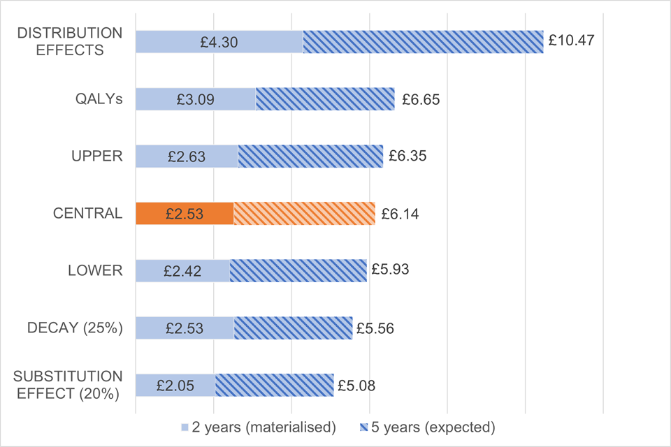
Figure 6.4: Exchequer benefit-cost ratios

Figure 6.5: DWP benefit-cost ratios

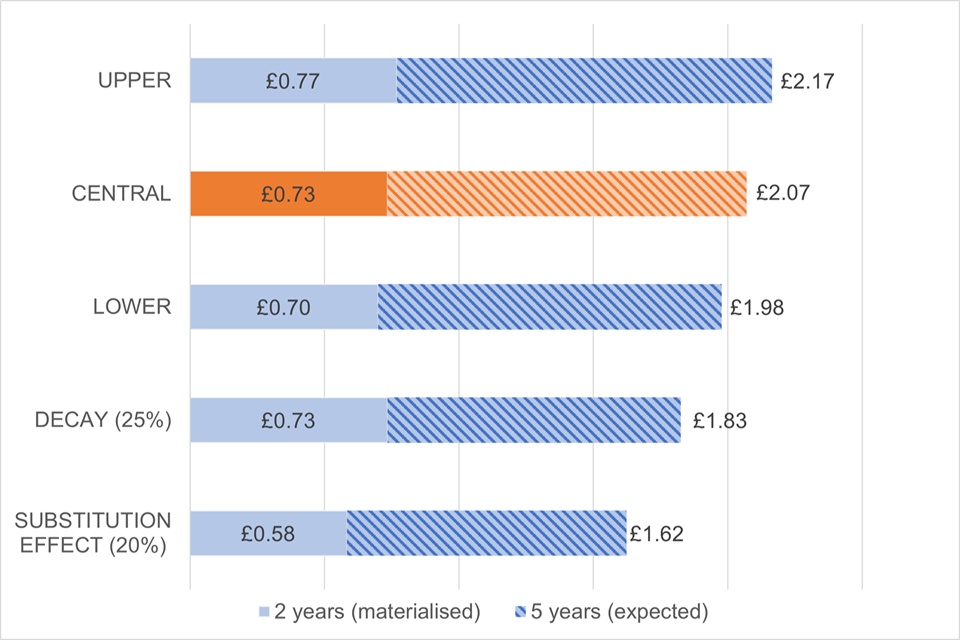
 6.3. Conclusions of the cost benefit analysis

We have used the estimated impact effects presented in section 5 and the DWP Social Cost‑Benefit Analysis framework to quantify the return on investment from the JETS programme under the participant, Exchequer, societal, and DWP perspectives. Results show that JETS generated a net gain to participants, the Exchequer, and society as early as 2 years after its implementation. Moreover, we expect a positive return for the DWP in a 5-year horizon. An assessment of the sensitivity of the results to varying model assumptions and the uncertainty in the impact estimates leaves the conclusion qualitatively unchanged.

In the baseline scenario and for each £1 spent in the programme, we estimate JETS generated a return of £1.34 to the Exchequer, £0.74 to the DWP, £2.53 to society and £2.07 to participants after the first 2 years. We expect the return to increase to £3.68 for the Exchequer, £2.07 to DWP, £6.14 to society and to be of £2.06 for participants in a 5 year horizon.

It is important to consider that the accuracy of these estimates depend on the robustness of the impact estimates from which they are derived, the validity of the assumptions on which they are based, and the underlying model assumptions of the CBA framework.

References

Caliendo, M., Mahlstedt, R. and Mitnik, O.A. (2014). Unobservable, but Unimportant? The Influence of Personality Traits (and other Usually Unobserved Variables) for the Evaluation of Labor Market Policies. DIW Berlin Discussion Paper No. 1407. http://dx.doi.org/10.2139/ssrn.2487797

Powell, A., Francis-Devine, B., Clark, H. (2022). Coronavirus: Impact on the labour market. House of Commons Library. Available at: Coronavirus: Impact on the labour market - House of Commons Library (parliament.uk) (accessed on 11/12/2024)

Fujiwara, D. (2010). The DWP Social Cost-Benefit Analysis framework (WP86). Department for Work and Pensions Working Paper 86. Available at: The DWP Social Cost-Benefit Analysis framework (WP86)

Department for Work and Pensions (2018). Universal Credit Programme Full Business Case Summary. Available at: Universal Credit Programme full business case summary - GOV.UK (www.gov.uk) (accessed on 11/12/2024)

Department for Work and Pensions (2024) Kickstart Scheme: A Quantitative Impact Assessment. DWP research report no. RR 1053. Available at: Kickstart Scheme: A Quantitative Impact Assessment - GOV.UK

House of Commons Work and Pensions Committee (2023). Plan for Jobs and employment support, Eighth Report of Session 2022–23. House of Commons. (https://committees.parliament.uk/publications/40930/documents/200444/default/, accessed on 28/03/2024).

Office for Budget Responsibility. (April 2020) “Commentary on the OBR coronavirus reference scenario.” Available at Commentary on the Public Sector Finances release (obr.uk) (accessed on 11/12/2024).

Schuring, M., Mackenbach, J., Voorham, T., & Burdorf, A. (2011). The effect of re-employment on perceived health. Journal of Epidemiology & Community Health, 65(7), 639-644. https://doi.org/10.1136/jech.2009.103838

Appendix A: Data

For this analysis we have created a unique dataset that combines multiple information obtained from several sources.

Provider Referrals and Payments system (PRaP)

PRaP is the tool used to administer contracted employment support programmes. From PRaP we identify the individuals referred to the scheme, the date of referral, participation status, and the contracted provider assigned. PRaP is also used to identify previous referrals or participation in other employment support schemes.

Real Time Information (RTI) data

RTI is the reporting system for income taxed via Pay-As-You-Earn (PAYE) managed by HMRC. Through RTI we capture the effective periods over which individuals have received income from payrolled employment. More information on how RTI can be used to derive earnings and periods of employment can be found here: Monthly earnings and employment estimates from Pay As You Earn Real Time Information (PAYE RTI) data: methods - Office for National Statistics (ons.gov.uk).

Department for Work and Pensions (DWP) benefit datasets

Information on out-of-work or low-income benefit receipt is obtained from either the UC Processing database – for Universal Credit related benefits – or from the National Benefits Database (NBD) – for all other benefits. These datasets are created by DWP and support the management of the benefit system.^{[footnote 37]}

These datasets further include other relevant personal characteristics like age, sex, whether living in partnership and/or with dependent children, among others. Additional information from individuals like ethnicity, socio-economic occupation, highest level of education attained, or disabilities are obtained from the Labour Market System (LMS). While not directly a benefit dataset, the LMS is used in Jobcentres to record and manage interactions between DWP and claimants.

The variables in these datasets contain missing values, often when filling in a particular field is optional. For variables where this occurs, we treat “missing” or “unknown” values as a valid category when controlling for participants characteristics.

Self Assessment tax returns

From the Self Assessment system – managed by HM Revenue and Customs (HMRC) and used to collect Income Tax – we derive self-reported periods in self‑employment before referral to the programme.

Local labour market environment

We merge information relating to the local labour market at the point of referral to JETS. More specifically, we use,

• Unemployment rate: from the Annual Population Survey and created by the ONS at the Jobcentre Plus district level
• Intensive work search rate: the number of individuals on UC with searching conditionality – obtained from Stat-Xplore at the Local Authority level – divided by the working age population (aged 16 to 64) – obtained from the ONS Population estimates at the local authority by five-year age bands
• Vacancy rate: The average number of job vacancies in each local authority area – obtained from Adzuna – divided by the number of individuals in UC with searching conditionality (from Stat-Xplore)

Appendix B: Additional Figures and Tables

Appendix Figure B.1: Programme effects on Looking for work benefits – Main sample

a) Proportion in category by group

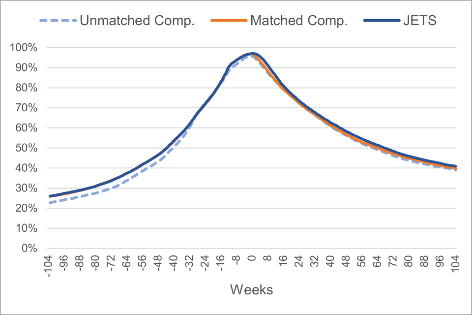
Panel a) of Figure B.1 shows there was a similar proportion of individuals in looking for work benefits between participants and matched non-participants over the 2 years prior to being referred to the programme. After referral, those who received support from the scheme were slightly more likely to be in looking for work benefits than those who did not (40.9% versus 39.9%, respectively, at year 2).

b) Percentage point difference

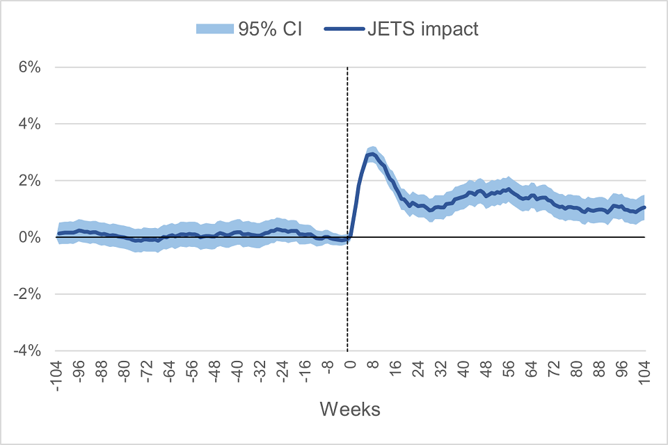
Panel b) of Figure B.1 shows there were no differences in looking for work benefit receipt between participants and matched non-participants over the 2 years prior to being referred to the programme. Since then, those who received support from the scheme were slightly more likely to be in looking for work benefits than those who did not (1.6 pp more likely at year 1 and 1.1 pp more likely at year 2). The light blue area represents the 95% confidence interval of the point estimates.

Appendix Figure B.2: Programme effects on Other out-of-work/low-income benefits – Main sample

a) Proportion in category by group

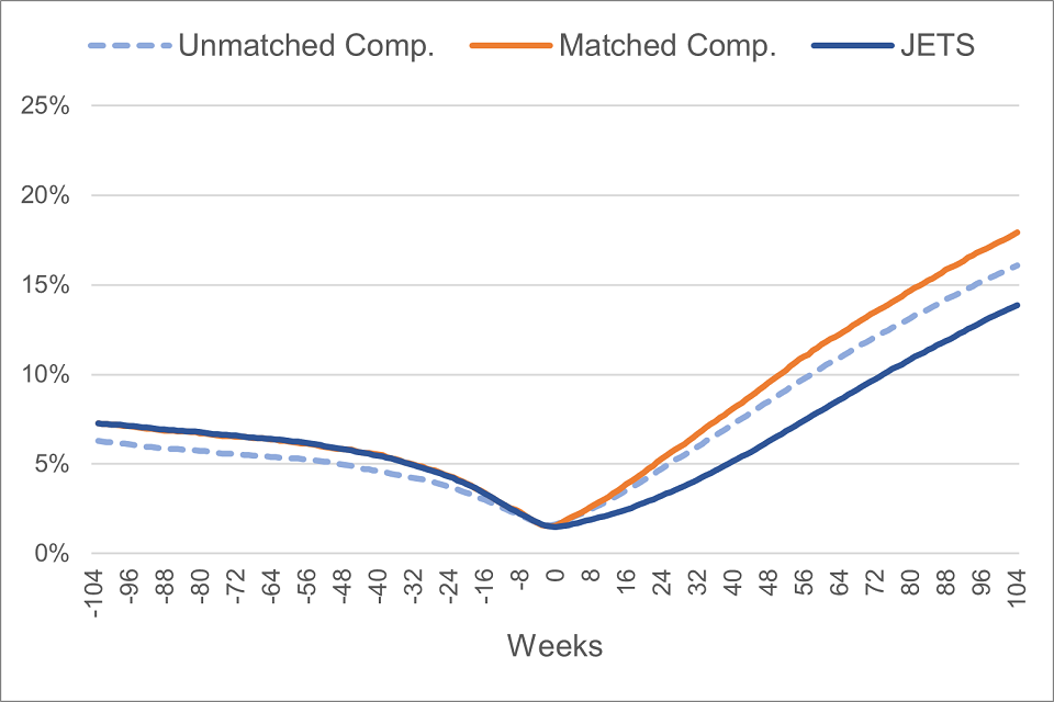
Panel a) of Figure B.2 shows there was a similar proportion of individuals in other out-of-work/low-income benefits between participants and matched non-participants over the 2 years prior to being referred to the programme. After referral, those who received support from the scheme were less likely to be in other out-of-work/low-income benefits than those who did not (13.9% versus 17.9%, respectively, at year 2).

b) Percentage point difference

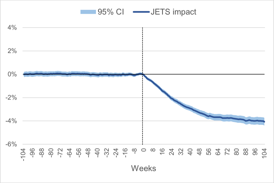
Panel b) of Figure B.2 shows there were no differences in other out-of-work/low-income benefit receipt between participants and matched non-participants over the 2 years prior to being referred to the programme. Since then, those who received support from the scheme were less likely to be in other out-of-work/low-income benefits than those who did not (3.4 pp less likely at year 1 and 4.1 pp less likely at year 2). The light blue area represents the 95% confidence interval of the point estimates.

Appendix Figure B.3: Programme effects on ‘Other’ category (not in employment nor on benefits) – Main sample

a) Proportion in category by group

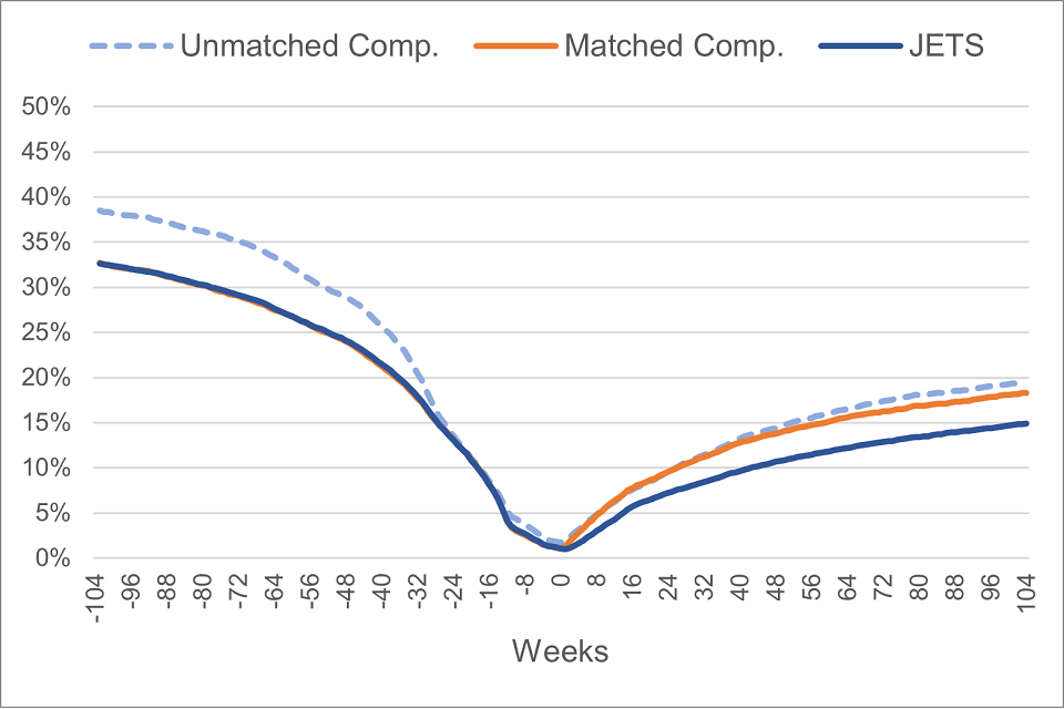
Panel a) of Figure B.3 shows there was a similar proportion of individuals in the ‘other’ category (not in employment nor on benefits) between participants and matched non-participants over the 2 years prior to being referred to the programme. After referral, those who received support from the scheme were less likely to be in the ‘other’ category than those who did not (14.9% versus 18.3%, respectively, at year 2).

b) Percentage point difference

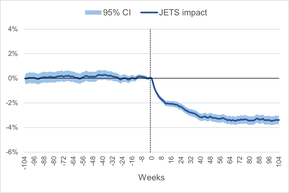
Panel b) of Figure B.3 shows there were no differences in the proportion of individuals in the ‘other’ category (not in employment nor on benefits) between participants and matched non-participants over the 2 years prior to being referred to the programme. Since then, those who received support from the scheme were less likely to be in the ‘other’ category than those who did not (3.2 pp less likely at year 1 and 3.4 pp less likely at year 2). The light blue area represents the 95% confidence interval of the point estimates.

Appendix Figure B.4: Programme effects on ‘In employment and not on benefits’ - Main sample

a) Proportion in category by group

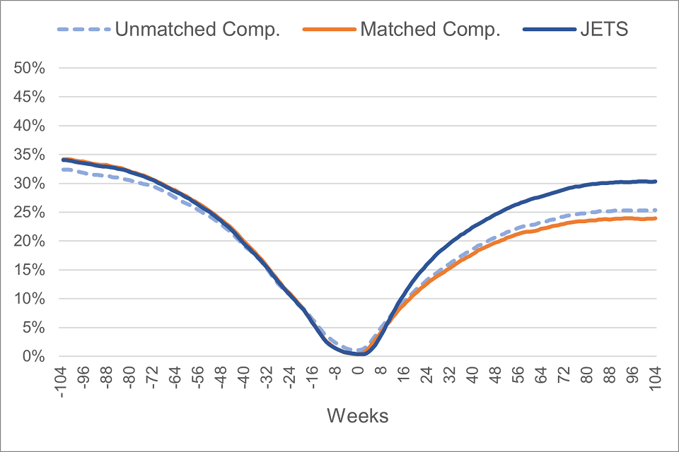
Panel a) of Figure B.4 shows there was a similar proportion of individuals in employment and not on benefits between participants and matched non-participants over the 2 years prior to being referred to the programme. After referral, those who received support from the scheme were more likely to be in employment and not on benefits than those who did not (30.3% versus 23.9%, respectively, at year 2).

b) Percentage point difference

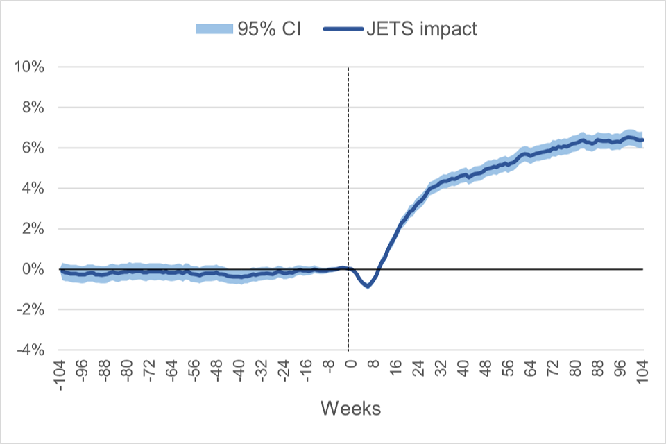
Panel b) of Figure B.4 shows there were no differences in the proportion of individuals in employment and not on benefits between participants and matched non-participants over the 2 years prior to being referred to the programme. Since then, those who received support from the scheme were more likely to be in employment and not on benefits than those who did not (5.0 pp more likely at year 1 and 6.4 pp more likely at year 2). The light blue area represents the 95% confidence interval of the point estimates.

Appendix Figure B.5: Difference in cumulative earnings (£)

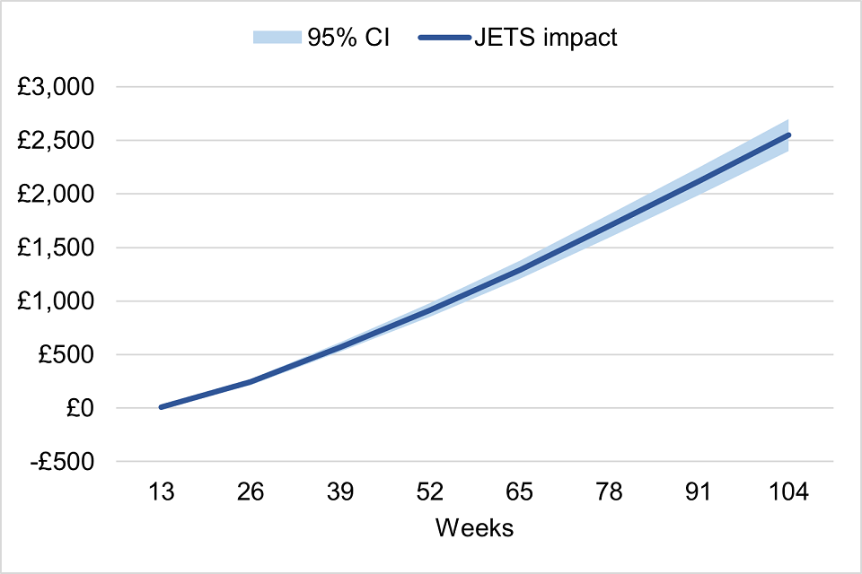
Figure B.5 displays the evolution in cumulative additional earnings from participating in JETS. The figure shows that, on average, those who started the programme had earned £ 915 in additional earnings by week 52, and £2,549 by week 104, relative to the comparison group.

Appendix Figure B.6: Percentage point difference in category – Early vs All Cohort (main sample)

Figure B.6 shows the percentage point difference in the proportion of individuals in looking for work benefits (panel a), other out-of-work/low-income benefits (panel b), other category (panel c), and in employment and not on benefits (panel d) over time between JETS participants and the matched comparison group for both the JETS All and the JETS Early cohorts. The figure displays similar impacts in the various labour market outcomes for both the All and the Early cohorts following participation in JETS.

a) Looking for work benefit

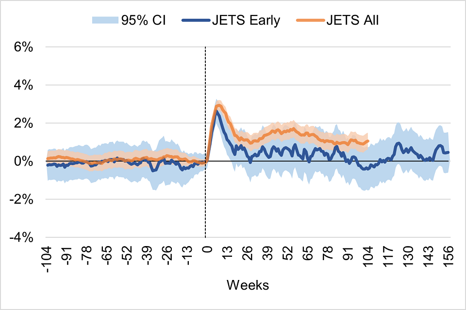
b) Other out-of-work/low-income benefit

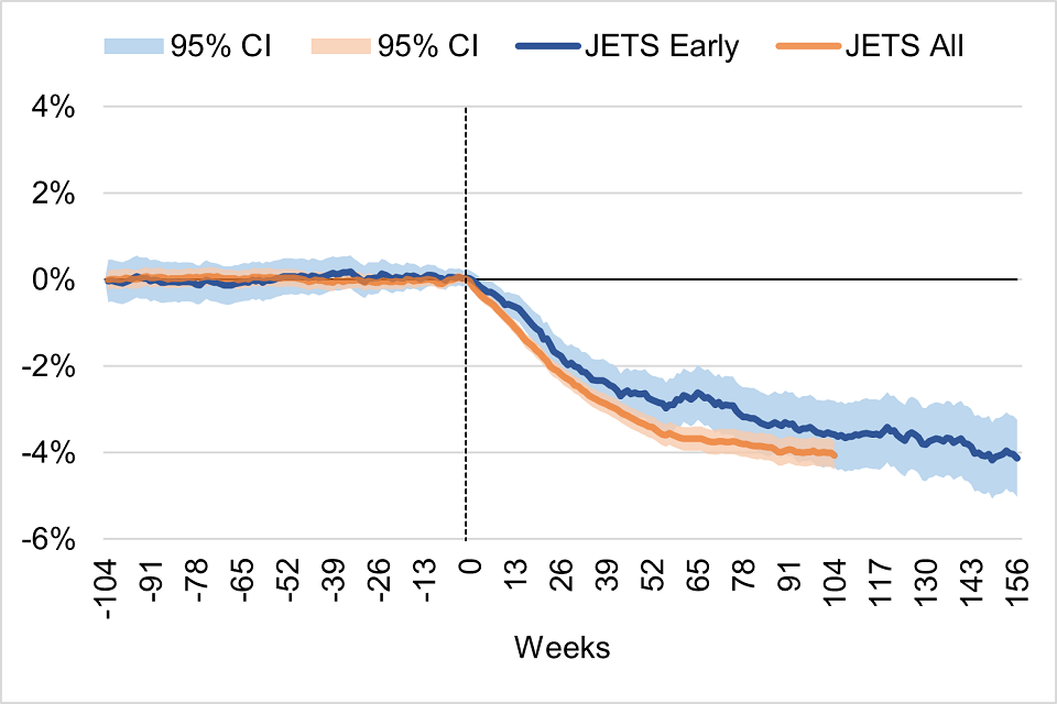
c) Other category

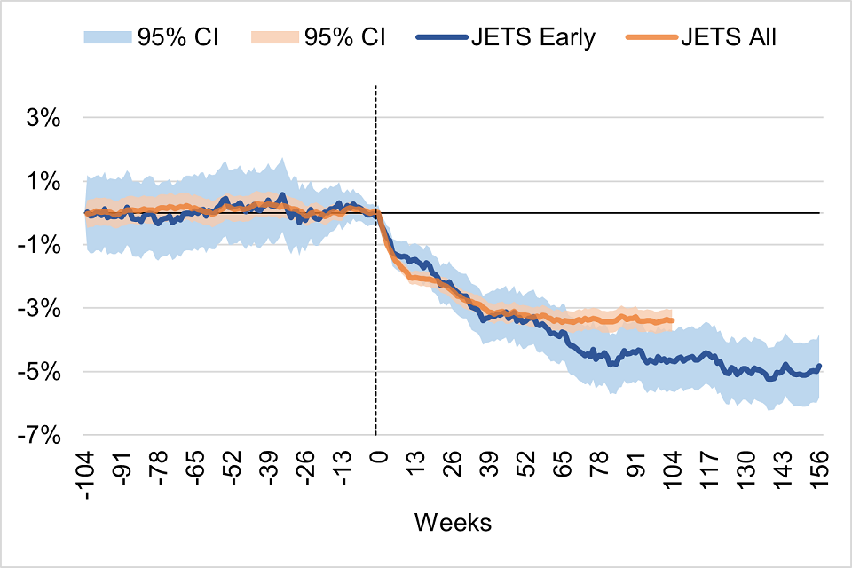
d) In employment and not on benefits

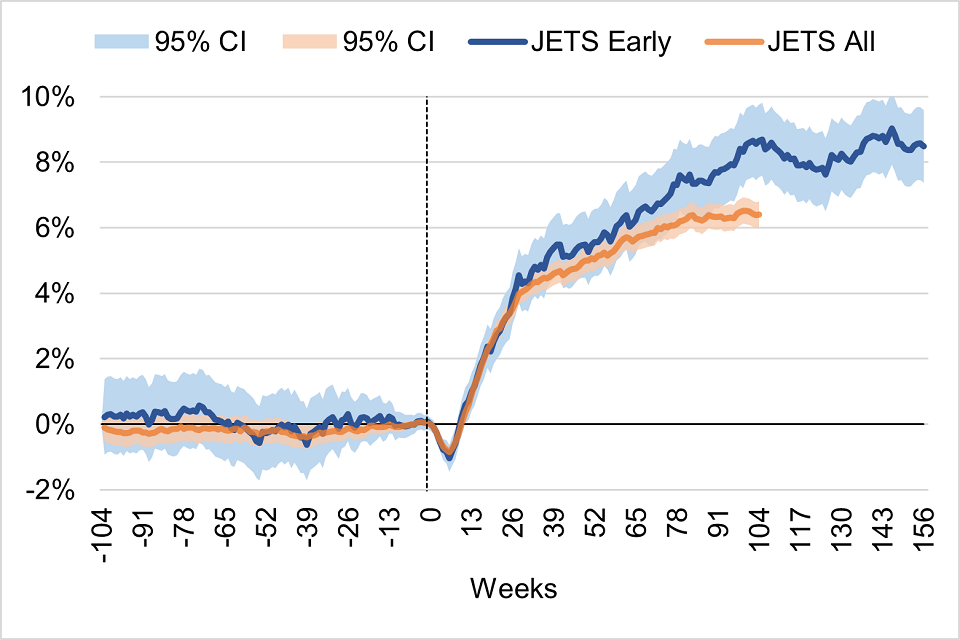
Appendix C: Long-term effects: Analysis of the Early cohort

Appendix Figure C.1: Common support – Early Cohort

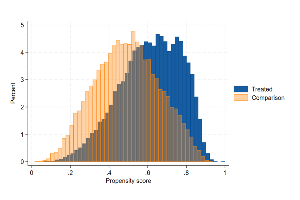
Figure C.1 displays the estimated propensity scores for the treatment and the comparison group in the Early Cohort sample. The two distributions are fairly similar and there exists good common support ranging approximately between 0.05 and 0.95.

Appendix Table C.1: Summary statistics of the matching exercise – Early Cohort

	Unmatched	Matched
Mean bias (%)	6.7	0.4
Median bias (%)	6.3	0.4
Max bias (%)	24.8	1.9
Rubin B	73.4	12.9
Rubin R	0.9	1.0

Appendix Figure C.2: Evolution in Payrolled employment – Early Cohort

a) Proportion in category by group

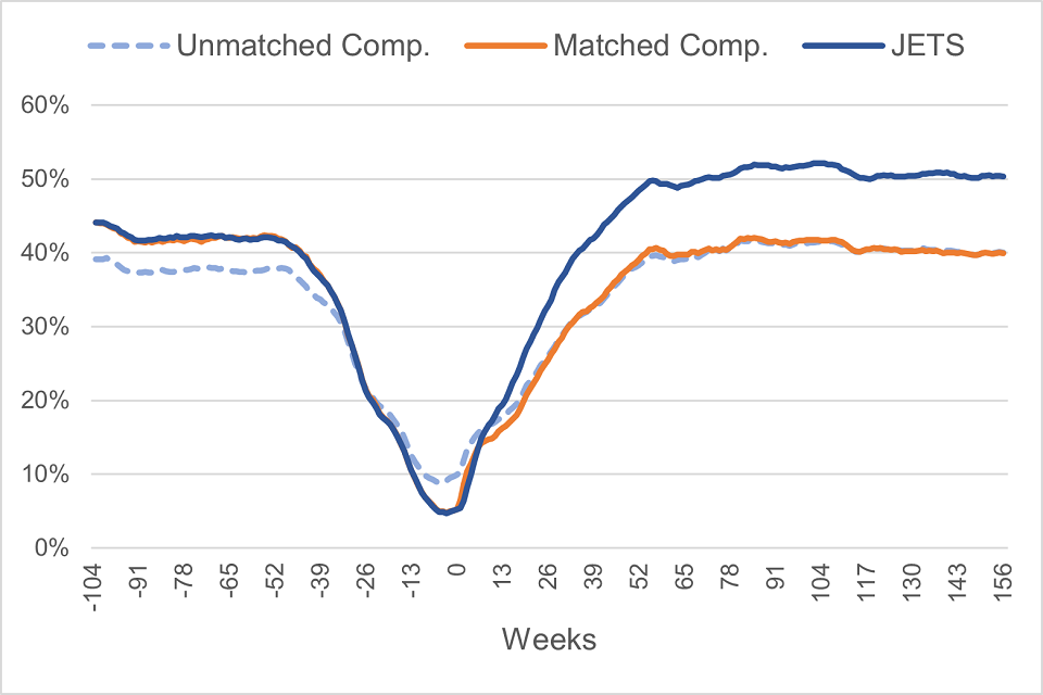
Panel a) of Figure C.2 shows that there was a similar proportion of individuals in payrolled employment between participants and matched non-participants from the Early cohort over the 2 years prior to being referred to the programme. After referral, those who received support from the scheme were more likely to be in payrolled employment than those who did not (50.3% versus 39.9%, respectively, at year 3).

b) Percentage point difference

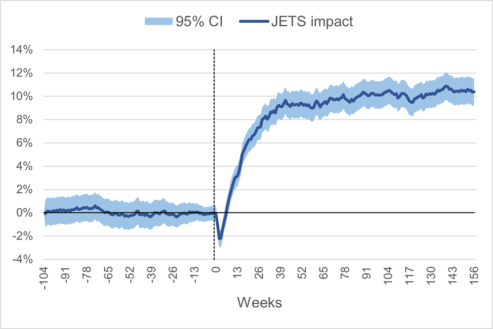
Panel b) of Figure C.2 shows there were no differences in payrolled employment between participants and matched non-participants from the Early Cohort over the 2 years prior to being referred to the programme. Since then and after a short ‘lock in’ effect period of lower employment, those who received support from the scheme were more likely to be in payrolled employment than those who did not (9.4 pp more likely at year 1, 10.5 pp more likely at year 2, and 10.4 pp more likely at year 3). The light blue area represents the 95% confidence interval of the point estimates.

Appendix Figure C.3: Evolution in Out-of-work benefits – Early Cohort

a) Proportion in category by group

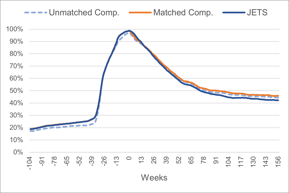
Panel a) of Figure C.3 shows there was a similar proportion of individuals in out-of-work or low income benefits between participants and matched non-participants from the Early Cohort over the 2 years prior to being referred to the programme. After referral, those who received support from the scheme were less likely to be in out-of-work or low income benefits than those who did not (42.2% versus 45.9%, respectively, at year 3).

b) Percentage point difference

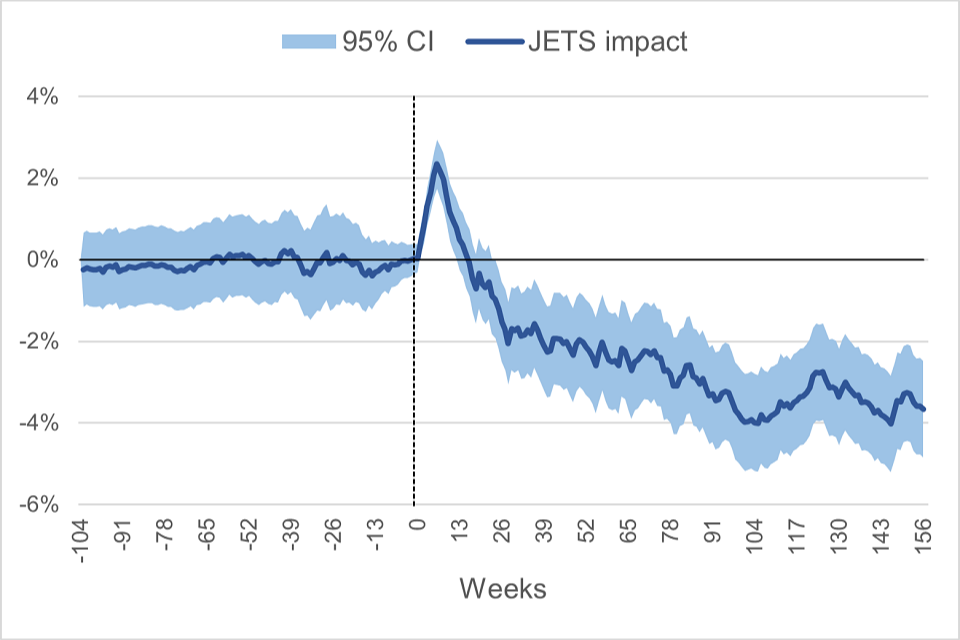
Panel b) of Figure C.3 shows there were no differences in out-of-work or low income benefit receipt between participants and matched non-participants from the Early Cohort over the 2 years prior to being referred to the programme. Since then and after a short ‘lock in’ effect period of higher benefit receipt, those who received support from the scheme were less likely to be in out-of-work or low income benefits than those who did not (2.1 pp less likely at year 1, 4.0 pp less likely at year 2, and 3.7 pp less likely at year 3). The light blue area represents the 95% confidence interval of the point estimates.

Appendix Figure C.4: Percentage point difference in category – Early Cohort

Figure C.4 shows the percentage point difference in the proportion of individuals in different labour market outcomes between participants and matched non-participants from the Early Cohort. All figures show no differences between groups over the two years leading to the referral. Three years after referral, there are no differences in the proportion of participants and matched non-participants in looking for work benefits (panel a), participants are less likely to be in other out-of-work/low-income benefits (4.1 pp, panel b) less likely to be in the other category (4.8 pp, panel c), and more likely to be in employment and not on benefits (8.5 pp, panel d) than the matched comparison group.

a) Looking for work benefit

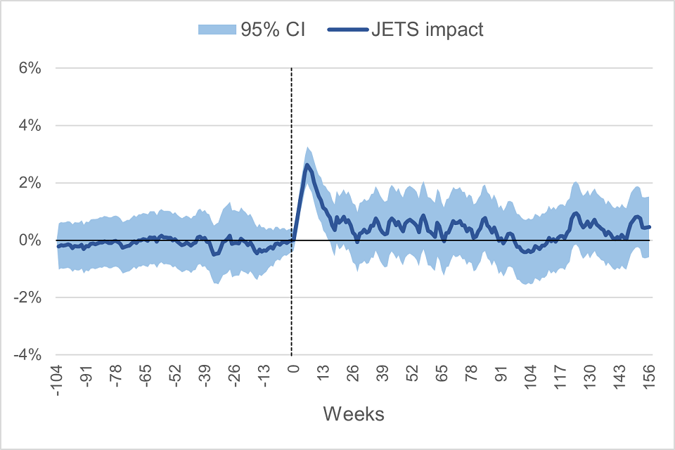
b) Other out-of-work/low-income benefit

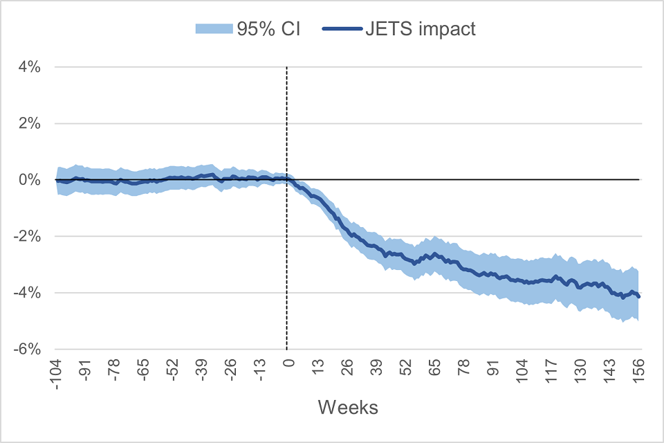
c) Other category

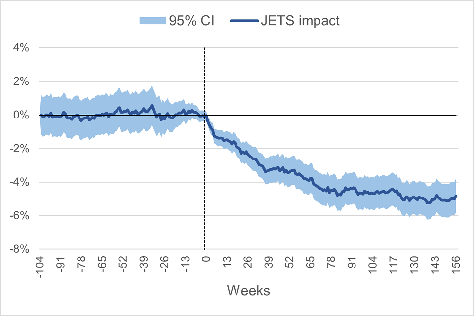
d) In employment and not on benefits

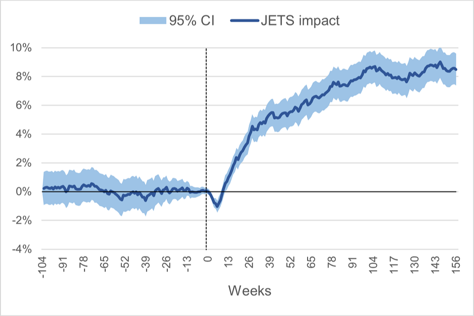
Appendix Table C.2: JETS impact over 3 years – Early Cohort

Payrolled employment	Treatment	Comparison	Impact [95% CI]
Days	482	387	95 [86 , 104]
Level (pp)	44.2	35.4	8.7 [7.9 , 9.6]

Earnings	Treatment	Comparison	Impact [95% CI]
Cumulative earnings (£)	24,902	19,567	5,335 [4,675 , 5,996]
Achieved £1K (pp)	72.8	62.3	10.6 [9.4 , 11.7]
Achieved £20K (pp)	45.7	35.9	9.9 [8.7 , 11.0]
Jobless	23.0	33.0	-10.0 [-11.1 , -9.0]

Out-of-work (OoW) benefits	Treatment	Comparison	Impact [95% CI]
Days	622	648	-26 [-35 , -17]
Level (pp)	56.9	59.3	-2.4 [-3.2 , -1.5]
Looking for work benefit: Days	539	534	5 [-3 , 13]
Looking for work benefit: Level (pp)	49.4	48.9	0.5 [-0.3 , 1.2]
Other OoW benefit: Days	82	113	-31 [-37 , -25]
Other OoW benefit: Level (pp)	7.5	10.4	-2.8 [-3.4 , -2.3]

Other category	Treatment	Comparison	Impact [95% CI]
Days	143	185	-42 [-49 , -35]
Level (pp)	13.1	16.9	-3.8 [-4.5 , -3.2]

Appendix Table C.3: Impact at each follow-up year – Early Cohort

Payrolled Employment (pp)	Baseline	Year 1	Year 2	Year 3
Treatment	5.2	48.5	52.2	50.3
Comparison	5.2	39.1	41.7	39.9
Impact [95% CI]	–	9.4 [8.2 , 10.5]	10.5 [9.3 , 11.7]	10.4 [9.2 , 11.6]

Out-of-Work (OoW) benefits (pp)	Baseline	Year 1	Year 2	Year 3
Treatment	98.7	58.6	44.7	42.2
Comparison	98.7	60.8	48.7	45.9
Impact [95% CI]	–	-2.1 [-3.3 , -1.0]	-4.0 [-5.2 , -2.8]	-3.7 [-4.8 , -2.5]
Looking for work benefit (pp): Treatment	98.1	54.0	34.6	27.6
Looking for work benefit (pp): Comparison	98.1	53.4	35.0	27.1
Looking for work benefit (pp): Impact [95% CI]	–	0.7 [-0.5 , 1.8]	-0.4 [-1.5 , 0.7]	0.5 [-0.6 , 1.5]
Other OoW benefit (pp): Treatment	0.6	4.6	10.1	14.6
Other OoW benefit (pp): Comparison	0.6	7.4	13.7	18.8
Other OoW benefit (pp): Impact [95% CI]	–	-2.8 [-3.4 , -2.2]	-3.6 [-4.4 , -2.8]	-4.1 [-5.0 , -3.2]

Other category (pp)	Baseline	Year 1	Year 2	Year 3
Treatment	0.9	11.9	16.6	18.9
Comparison	1.0	15.3	21.3	23.8
Impact [95% CI]	–	-3.4 [-4.3 , -2.6]	-4.7 [-5.6 , -3.7]	-4.8 [-5.8 , -3.8]

Appendix D: Analysis with alternative model specifications

This section inspects the sensitivity of the main impact estimates to different model specifications.

Appendix Table D.1 shows a summary of impact results after estimating the following models:

• Base model (main estimates): Nearest neighbour matching to 4 non-participants allowing for replacement, propensity score estimated using a logit model, calliper width of 0.01
• Model 1: Estimating an OLS regression of labour market outcomes on the treatment using the base matched sample (described above), controlling for the matching variables, and clustering the standard errors at the individual level (double robust estimator)
• Model 2: Nearest neighbour matching to 1 non-participant allowing for replacement, propensity score estimated using a logit model, calliper width of 0.001
• Model 3: Base model but applying a more parsimonious specification in the logit model (see Appendix E for more detail)
• Model 4: Nearest neighbour matching to 4 non-participants allowing for replacement, propensity score estimated using a probit model, calliper width of 0.01

All in all, results show impact estimates are robust to alternative model specifications and the use of alternative PSM parameters. Moreover, all models are within the commonly accepted thresholds that determine success of the matching algorithm:

• Common support close to 100%
• Rubin B ranges from 4.7 to 8.1
• Rubin R is fixed at 1.0
• Median bias ranges from 0.23 to 0.30
• Maximum % bias is between 1.4 and 1.7

Appendix Table D.1 shows that, depending on the model used, JETS participants were between 8.8 pp and 8.9 pp more likely to be employed two years after being referred and between 3.0 pp and 3.2 pp less likely to be on an out-of-work or low‑income benefit than non-participants. Overall, those starting JETS spent between 52 and 54 additional days in employment and between 11 and 13 fewer days on an unemployment related benefit. The additional earnings from participating in JETS are estimated to vary between £2,549 and £2,700 two years after programme start, with those receiving support from the scheme less likely to be in the ‘Other’ category (not in employment nor on benefits) by the end of the observation period (between 3.1 pp and 3.2 pp less likely).

Appendix Table D.1: Sensitivity of impact estimates to alternative model specifications

Model	Base	Model 1	Model 2	Model 3	Model 4
Propensity score	Logit	Logit	Logit	Logit (pars)	Probit
N comparisons (k)	4	4	1	4	4
Caliper width	0.01	0.01	0.001	0.01	0.01
Double robust estimator	No	Yes	No	No	No
Rubin B	5.9	5.9	8.1	4.7	6.0
Rubin R	1.0	1.0	1.0	1.0	1.0
Mean % bias	0.31	0.31	0.32	0.31	0.27
Median % bias	0.30	0.30	0.28	0.26	0.23
Max % bias	1.6	1.6	1.7	1.4	1.7
Off support	1	1	35	31	0

Employment	Base	Model 1	Model 2	Model 3	Model 4
Year 1 (pp)	8.2 (0.22)	8.2 (0.21)	8.1 (0.26)	8.3 (0.22)	8.2 (0.22)
Year 2 (pp)	8.8 (0.22)	8.8 (0.21)	8.8 (0.27)	8.9 (0.22)	8.9 (0.22)
Additional days	52.7 (1.2)	53.1 (1.1)	52.6 (1.4)	53.9 (1.2)	52.7 (1.2)
Additional earnings (£)	2,549 (76.7)	2,590 (67.7)	2,534 (89.9)	2,700 (75.3)	2,586 (76.6)

OoW benefits	Base	Model 1	Model 2	Model 3	Model 4
Year 1 (pp)	-1.8 (0.22)	-1.9 (0.20)	-1.8 (0.26)	-1.9 (0.22)	-1.9 (0.22)
Year 2 (pp)	-3.0 (0.23)	-3.1 (0.21)	-3.1 (0.27)	-3.2 (0.23)	-3.2 (0.23)
Additional days	-11.3 (1.2)	-12.1 (1.0)	-11.4 (1.4)	-12.2 (1.1)	-12.1 (1.2)

Looking for work benefits	Base	Model 1	Model 2	Model 3	Model 4
Year 1 (pp)	1.6 (0.23)	1.4 (0.22)	1.6 (0.27)	1.5 (0.23)	1.5 (0.23)
Year 2 (pp)	1.1 (0.23)	0.9 (0.22)	1.0 (0.27)	0.9 (0.22)	0.9 (0.23)
Additional days	10.1 (1.1)	9.0 (1.0)	10.4 (1.4)	9.2 (1.1)	9.5 (1.1)

Other OoW benefits	Base	Model 1	Model 2	Model 3	Model 4
Year 1 (pp)	-3.4 (0.13)	-3.4 (0.13)	-3.5 (0.16)	-3.4 (0.13)	-3.4 (0.13)
Year 2 (pp)	-4.1 (0.17)	-4.0 (0.17)	-4.1 (0.20)	-4.1 (0.16)	-4.1 (0.17)
Additional days	-21.4 (0.7)	-21.1 (0.7)	-21.8 (0.9)	-21.4 (0.7)	-21.6 (0.7)

Other category	Base	Model 1	Model 2	Model 3	Model 4
Year 1 (pp)	-3.2 (0.18)	-3.2 (0.16)	-3.2 (0.21)	-3.2 (0.18)	-3.1 (0.18)
Year 2 (pp)	-3.2 (0.18)	-3.2 (0.16)	-3.2 (0.21)	-3.2 (0.18)	-3.1 (0.18)
Additional days	-21.0 (0.8)	-20.7 (0.8)	-20.5 (1.0)	-20.9 (0.8)	-20.0 (0.8)

Standard errors in parenthesis.

Appendix E: Analysis with an alternative comparison sample

Our main estimation of programme effects compares the labour market outcomes of those who started JETS with a comparison group created from those who did not start the programme after being referred to it. Following this approach ensures that those in the comparison group:

• were considered suitable to join the scheme by Work Coaches in JCP
• had shown interest in participating in JETS (although did not start the provision)

In this section, instead, we derive programme effects by creating a comparison group from a random sample of individuals claiming UC-IWS that were never referred to the scheme. The random sample is drawn among those who had a benefit assessment that fell within the period in which JETS was accepting referrals.^{[footnote 38]} As this group was never referred, we derive a pseudo-referral date using the benefit assessment date and select individuals to match the distribution of ‘real’ referral dates to JETS.

Estimating the programme’s counterfactual from a sample of non-referred individuals has the advantage of removing the selection bias that might arise when deciding (or being able) to start the programme.^{[footnote 39]} On the other hand, those who were never referred to the scheme might differ from JETS participants (in both observables and unobservable characteristics) in a higher magnitude than those who were referred but did not start the provision. For instance, individuals not referred to JETS might have been considered unsuitable by Work Coaches in JCP or might have refused to be referred to the provision altogether (showing a lack of interest in participating).

As a matter of fact, Appendix Figure E.1 shows that the pre-matching evolution in payrolled employment of the referred not started group follows more closely that of the participant group than the non-referred group does. While the gap closes near the referral date – individuals become eligible –, the non-referred group had a much lower participation rate in the labour market than the referred not started group over the 2 years pre-intervention. Appendix Figure E.2, on the other hand, shows a closer similitude across groups in the evolution of out-of-work benefit receipt. Nevertheless, the trend on benefit receipt among those referred to the scheme that did not start is still more similar to the one of participants during the pre-intervention period.

In addition, the analysis of characteristics shows that the referred not started group is more similar to the participant group in observed attributes than those never referred to the scheme. This can be inferred from Appendix Table E.1 below, which shows the proportion of covariates that are unbalanced before and after the matching based on standardised mean differences or t-tests of mean differences for the sample of individuals referred to the scheme and not starting and the sample of those never referred. While the p-value results in the referred sample are in line with expectations after the matching, the p-values in the non-referred sample suggest imbalance.

Appendix Table E.1: Proportion of unbalanced covariates (before and after the matching) using the referred not started sample or the sample of non-referred individuals

	Standardised mean difference (%) outside the [-3%,3%] range: Unmatched	Standardised mean difference (%) outside the [-3%,3%] range: Matched	t-test of mean difference p-value < 0.05: Unmatched	t-test of mean difference p-value < 0.05: Matched
Referred sample	64.0%	0.0%	91.6%	7.1%
Non-referred sample	73.5%	2.0%	92.1%	23.2%

Appendix Figure E.1: Pre-programme and pre-matching trends in payrolled employment (proportion) by group

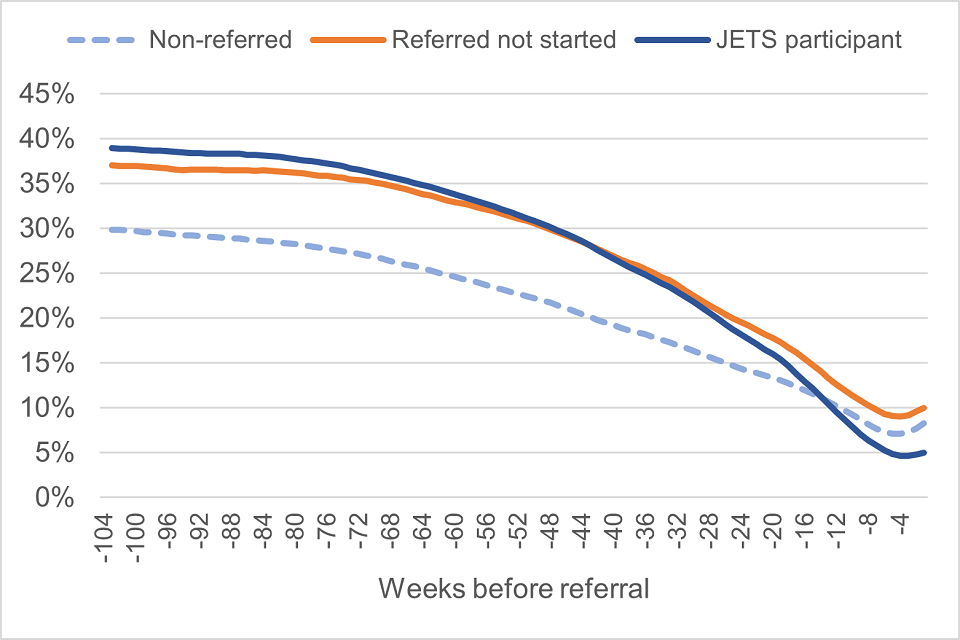
Figure E.1 displays the pre-matching evolution in payrolled employment among JETS participants, those referred to the programme who did not start, and those non-referred over the 2 years before referral (or pseudo-referral). The figure shows very similar payrolled employment levels over time between JETS participants and those refereed and not started, and substantially lower employment levels for the group of those never referred to the scheme.

Appendix Figure E.2: Pre-programme and pre-matching trends on out-of-work benefits (proportion) by group

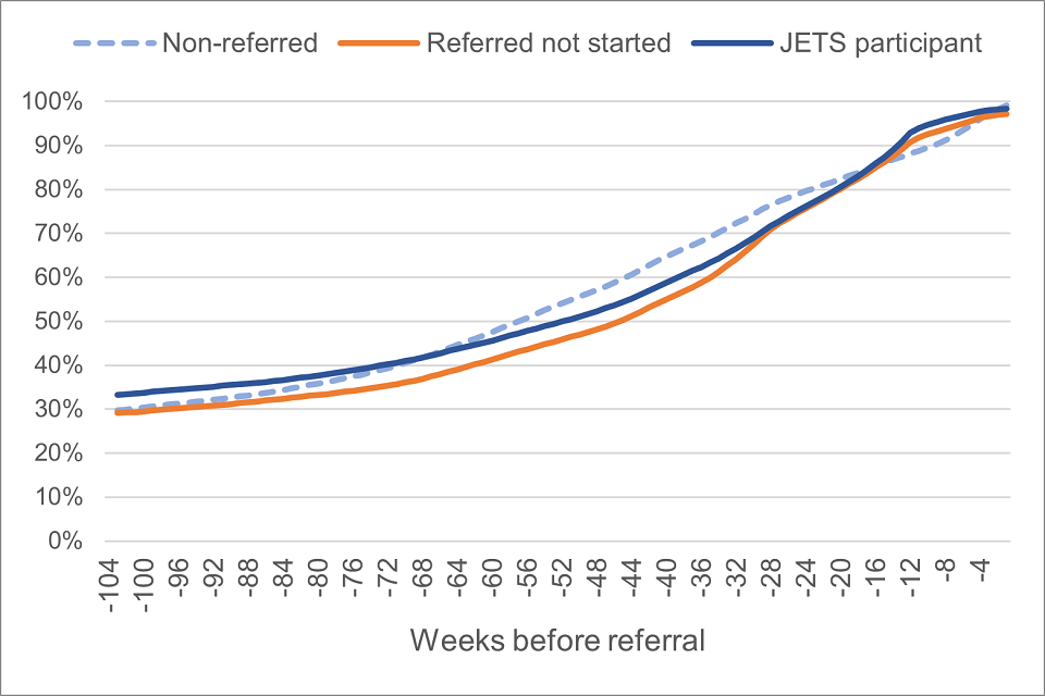
Figure E.2 displays the pre-matching evolution in out-of-work/low-income benefits among JETS participants, those referred to the programme who did not start, and those non-referred over the 2 years before referral (or pseudo-referral). The figure shows a similar evolution in the receipt of out-of-work/low-income benefits over time across all three groups.

Finally, a PSM analysis that compares the outcomes of those who were referred to JETS but did not start against those who were not referred to the scheme (B vs C in Appendix Figure E.3 below) shows a 5 pp employment rate difference (when we should expect no difference). We believe this is attributable to there being additional unobserved variables which affect the referral process.

Appendix Figure E.3: Analysis samples

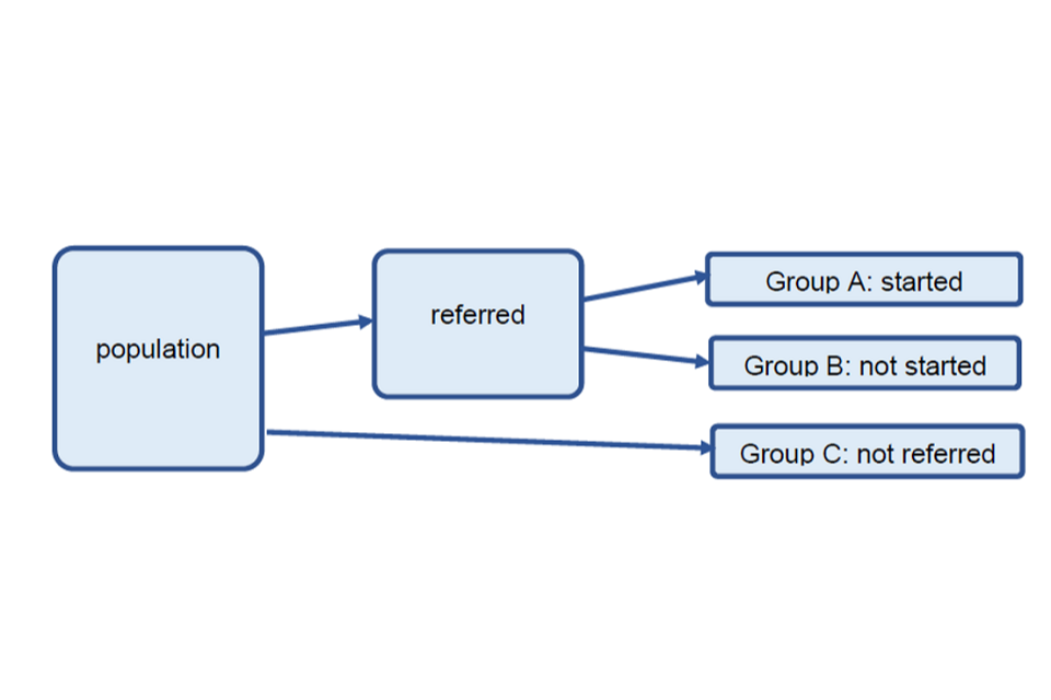
Figure E.3 shows how the population of interest in our analysis is split into three different groups: Group A (referred to JETS and starting the programme), Group B (referred to JETS and not starting the programme) and Group C (not referred to JETS).

For all the reasons above, we prefer to use the sample of individuals that were referred to JETS but did not start to derive our main comparison group for the estimation of programme effects.

Results with an alternative (non-referred) comparison sample

Appendix Figure E.4 shows significantly higher impact estimates from participating in JETS when using the non-referred sample to draw a matched comparison group.

Similarly, Appendix Figure E.5 shows a quicker reduction in the receipt of out-of-work or low-income benefits. While the reduction in the proportion of individuals receiving benefits is estimated to be similar using both approaches two years after programme start, this is the result of a very different evolution of the type of benefit received. The non-referred PSM impact estimates would suggest a higher increase in the proportion of individuals receiving a looking for work benefit and a higher reduction in the proportion of those receiving other out-of-work/low-income benefits following participating in JETS (see Appendix Figure E.6).

Appendix Figure E.4: Percentage point difference in payrolled employment – Non-referred vs Referred not started matched comparison sample

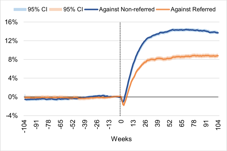
Figure E.4 shows a higher estimated impact in payrolled employment when using the non-referred group to construct the comparison sample than when using the referred not started group.

Appendix Figure E.5: Percentage point difference on out-of-work benefits – Non-referred vs Referred not started matched comparison sample

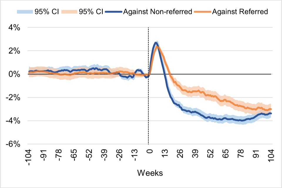
Figure E.5 shows a higher estimated reduction in the receipt of out-of-work/low-income benefits when using the non-referred group to construct the matched comparison sample than when using the referred not started group.

Appendix Figure E.6: Percentage point difference in category – Referred vs Non-referred comparison sample

Figure E.6 shows that when using the sample of non-referred individuals to construct the comparison group instead of the sample of those referred who do not start, we estimate a larger increase in the receipt of looking for work benefits after participation (Panel a), a larger decrease in the proportion of individuals in other out-of-work/low-income benefits (Panel b), a larger decrease in the likelihood of being in the other category (Panel c) and a larger increase in the proportion of individuals in employment and not on benefits (Panel d).

a) Looking for work benefit

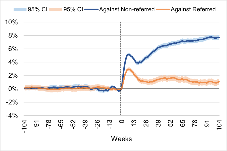
b) Other out-of-work/low-income benefit

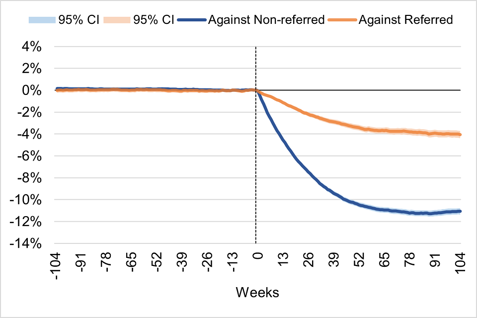
c) Other category

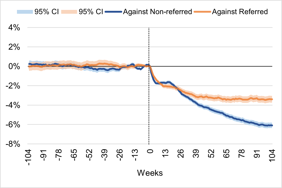
d) In employment and not on benefits

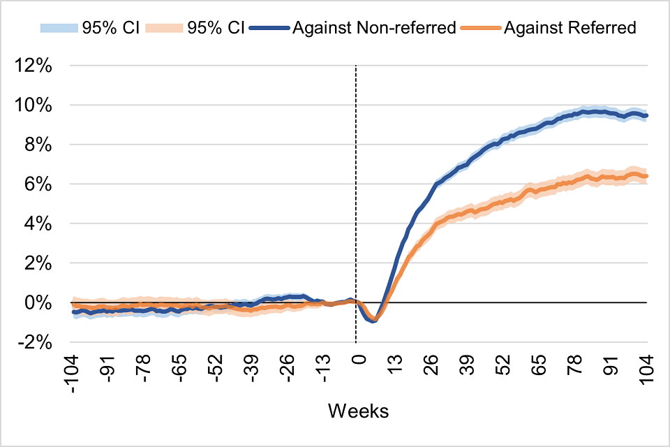
On average and over the span of 2 years, impact estimates in payrolled employment are estimated to be 4.8 pp higher when using the matched non-referred group (instead of the matched referred not started group), and the reduction in out-of-work benefit receipt is estimated to be 1.2 pp larger (see Appendix Table E.2).

Appendix Table E.2: JETS impact over 2 years – Non-referred vs Referred not started (main sample) estimates

Payrolled employment	Against non-referred: Impact [95% CI]	Against referred: Impact [95% CI]
Days	87 [86 , 89]	53 [50 , 55]
Level (pp)	12.0 [11.8 , 12.3]	7.2 [6.9 , 7.6]

Earnings	Against non-referred: Impact [95% CI]	Against referred: Impact [95% CI]
Cumulative earnings (£)	3,842 [3,727 , 3,957]	2,549 [2,399 , 2,699]
Achieved £1K (pp)	17.2 [16.8 , 17.6]	10.3 [9.8 , 10.7]
Achieved £20K (pp)	8.8 [8.5 , 9.1]	5.8 [5.4 , 6.1]
Jobless	-17.5 [-17.8 , -17.1]	-10.2 [-10.7 , -9.8]

Out-of-work (OoW) benefits	Against non-referred: Impact [95% CI]	Against referred: Impact [95% CI]
Days	-20 [-22 , -19]	-11 [-14 , -9]
Level (pp)	-2.8 [-3.0 , -2.6]	-1.6 [-1.9 , -1.2]
Looking for work benefit: Days	45 [44 , 47]	10 [8 , 12]
Looking for work benefit: Level (pp)	-9.0 [-9.2 , -8.8]	-2.9 [-3.1 , -2.7]

Other category	Against non-referred: Impact [95% CI]	Against referred: Impact [95% CI]
Days	-30 [-31 , -29]	-21 [-23 , -19]
Level (pp)	-4.1 [-4.3 , -3.9]	-2.9 [-3.1 , -2.7]

Appendix Figure E.7: Common support – PSM with Non-referred sample

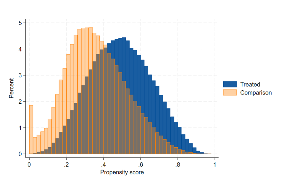
Figure E.7 displays the estimated propensity scores for the treatment and the comparison group when using the non-referred sample to construct the comparison group. The figure shows there exists good common support ranging approximately between 0 and 0.95, with a large mass of estimated values in the first bin (between 0 and 0.02) in the comparison group (close to 19%).

Appendix Table E.3: Summary statistics of the matching exercise – PSM with Non-referred sample

	Unmatched	Matched
Mean bias (%)	8.9	0.5
Median bias (%)	6.6	0.4
Max bias (%)	23.7	1.6
Rubin B	74.0	5.2
Rubin R	0.5	1.0

Appendix F: Estimating the propensity score

We use two alternative set of matching covariates to estimate the propensity score to participate in JETS:

• Main (referred sample) specification. This is our main specification, used in the PSM analysis that constructs the comparison group from those individuals who were referred to the scheme but did not start.
• Parsimonious (UC-IWS wider sample) specification. This is the specification used in the PSM analysis when constructing the comparison group from those individuals in UC-IWS that were never referred to the scheme. This specification is also used in the main (referred) sample to assess the sensitivity of the impact estimates to a more parsimonious specification of the logit model.^{[footnote 40]}

Appendix Table F.1: Detailed list of matching variables

Matching variables (over 2 years before referral)	Main (referred sample) specification	Parsimonious (UC-IWS wider sample) specification
In payrolled employment	Weekly flags	Quarterly flags
On out-of-work benefits	Weekly flags	Quarterly flags
Looking for work benefit	Quarterly flags	Quarterly flags
Not in employment nor on out-of-work benefits	Quarterly flags	Quarterly flags
Labour market transitions 13 weeks before referral (Employment-Benefits-Other)	Y	Y
Cumulative days in payrolled employment	Quarterly	Quarterly
Cumulative days on out-of-work benefits	Quarterly	Quarterly
Cumulative days on looking for work benefit	Quarterly	Quarterly
Cumulative days on Other out-of-work/low-income benefits	Quarterly	Quarterly
Cumulative days not in employment nor on out-of-work benefits	Quarterly	Quarterly
Cumulative days in self-employment	Quarterly	-
Cumulative days in DLA-PIP benefit	Quarterly	-
Inverse hyperbolic sine of earnings	Quarterly	Quarterly
Individual information exists in client dataset	Y	Y
Male	Y	Y
Age (continuous)	Y	Y
Age groups	Y	Y
Any disability	Y	Y
15 variables on type of disability	Y	-
Ethnicity categories	Y	Y
Lone parent	Y	Y
Parent	Y	Y
Refugee	Y	-
Homeless	Y	-
Socio-economic occupations	Y	Y
JCP district dummies	Y	Y
Date of referral	Y	Y
Intensive work search rate	Y	-
Unemployment rate	Y	-
Vacancy rate	Y	-
p14 earnings from previous tax years	Y	-
Referred to Work Programme	Y	Y
Started Work & Health Programme	Y	-
Started other Contracted Employment support	Y	Y

Appendix G: Extended list of covariates balance

Appendix Table G.1: Extended summary of covariates balance

Variable	Sample	Treatment	Comparison	% Bias	Reduction	t-stat	p-value
Male	Unmatched	0.58	0.60	-3.4	–	-9.05	0.00
Male	Matched	0.58	0.58	0.0	98.9%	-0.12	0.90
Age	Unmatched	38.2	37.3	7.3	–	19.39	0.00
Age	Matched	38.2	38.2	-0.3	95.6%	-1.02	0.31
Age group: 18-24	Unmatched	0.11	0.13	-6.7	–	-17.98	0.00
Age group: 18-24	Matched	0.11	0.11	0.4	93.9%	1.35	0.18
Age group: 25-49	Unmatched	0.67	0.66	0.6	–	1.70	0.09
Age group: 25-49	Matched	0.67	0.67	-0.1	85.0%	-0.31	0.76
Age group: 50+	Unmatched	0.22	0.20	4.8	–	12.59	0.00
Age group: 50+	Matched	0.22	0.22	-0.2	95.4%	-0.69	0.49
Disabled	Unmatched	0.15	0.14	2.8	–	7.38	0.00
Disabled	Matched	0.15	0.15	-0.4	83.9%	-1.41	0.16
Disability: Mobility	Unmatched	0.03	0.03	0.8	–	2.03	0.04
Disability: Mobility	Matched	0.03	0.03	0.1	91.8%	0.20	0.84
Disability: Manual Dexterity	Unmatched	0.01	0.01	1.0	–	2.75	0.01
Disability: Manual Dexterity	Matched	0.01	0.01	-0.3	75.8%	-0.78	0.44
Disability: Physical Coordination	Unmatched	0.01	0.01	0.1	–	0.28	0.78
Disability: Physical Coordination	Matched	0.01	0.01	-0.3	-149.5%	-0.82	0.41
Disability: Continence	Unmatched	0.00	0.00	0.5	–	1.30	0.19
Disability: Continence	Matched	0.00	0.00	-0.22	55.8%	-0.67	0.50
Disability: Lift/carry/move objects	Unmatched	0.03	0.03	0.32	–	0.85	0.40
Disability: Lift/carry/move objects	Matched	0.03	0.03	-0.30	5.6%	-0.96	0.34
Disability: Speech, hearing or vision	Unmatched	0.01	0.01	1.58	–	4.13	0.00
Disability: Speech, hearing or vision	Matched	0.01	0.01	-0.28	82.3%	-0.85	0.40
Disability: Memory, concentration, learning	Unmatched	0.05	0.05	2.31	–	6.07	0.00
Disability: Memory, concentration, learning	Matched	0.05	0.05	-0.09	96.0%	-0.29	0.77
Disability: Perception of risk, danger	Unmatched	0.00	0.00	-0.1	–	-0.19	0.85
Disability: Perception of risk, danger	Matched	0.00	0.00	0.3	-276.4%	0.85	0.40
Disability: Cumulative effect of above	Unmatched	0.04	0.04	0.3	–	0.67	0.50
Disability: Cumulative effect of above	Matched	0.04	0.04	-0.1	76.4%	-0.19	0.85
Disability: past Disability	Unmatched	0.02	0.02	0.0	–	-0.02	0.98
Disability: past Disability	Matched	0.02	0.02	0.4	-4956.2%	1.39	0.16
Disability: Progressive Condition	Unmatched	0.01	0.01	0.0	–	-0.01	0.99
Disability: Progressive Condition	Matched	0.01	0.01	-0.4	-13481.3%	-1.28	0.20
Disability: Recurring Condition	Unmatched	0.06	0.05	1.5	–	3.94	0.00
Disability: Recurring Condition	Matched	0.06	0.06	-0.3	77.3%	-1.06	0.29
Disability: Severe Disfigurement	Unmatched	0.00	0.00	-0.3	–	-0.86	0.39
Disability: Severe Disfigurement	Matched	0.00	0.00	0.1	76.1%	0.26	0.80
Disability: Existing PWD client	Unmatched	0.00	0.00	-0.5	–	-1.26	0.21
Disability: Existing PWD client	Matched	0.00	0.00	-0.6	-32.5%	-1.96	0.05
Disability: Special Support	Unmatched	0.00	0.00	1.3	–	3.34	0.00
Disability: Special Support	Matched	0.00	0.00	0.1	88.6%	0.44	0.66
Lone parent	Unmatched	0.11	0.09	4.2	–	11.11	0.00
Lone parent	Matched	0.11	0.11	0.3	92.7%	0.96	0.34
Parent	Unmatched	0.16	0.14	5.1	–	13.46	0.00
Parent	Matched	0.16	0.15	0.3	94.3%	0.92	0.36
Missing parenthood	Unmatched	0.12	0.12	-0.9	–	-2.51	0.01
Missing parenthood	Matched	0.12	0.12	0.3	67.9%	0.98	0.33
Refugee	Unmatched	0.01	0.01	-0.2	–	-0.52	0.60
Refugee	Matched	0.01	0.01	0.5	-154.7%	1.63	0.10
Homeless	Unmatched	0.00	0.01	-2.4	–	-6.68	0.00
Homeless	Matched	0.00	0.00	0.1	96.1%	0.34	0.74
SOC: Missing	Unmatched	0.45	0.48	-6.7	–	-17.73	0.00
SOC: Missing	Matched	0.45	0.45	0.3	95.3%	0.99	0.32
SOC: Managers and Senior Officials	Unmatched	0.03	0.02	4.5	–	11.68	0.00
SOC: Managers and Senior Officials	Matched	0.03	0.03	-0.04	99.2%	-0.11	0.91
SOC: Professional Occupations	Unmatched	0.01	0.01	2.50	–	6.51	0.00
SOC: Professional Occupations	Matched	0.01	0.01	-0.25	90.2%	-0.74	0.46
SOC: Associate Professional and Technical Occupations	Unmatched	0.03	0.03	1.67	–	4.41	0.00
SOC: Associate Professional and Technical Occupations	Matched	0.03	0.03	0.50	70.1%	1.57	0.12
SOC: Administrative and Secretarial Occupations	Unmatched	0.06	0.05	4.46	–	11.68	0.00
SOC: Administrative and Secretarial Occupations	Matched	0.06	0.06	-0.14	96.8%	-0.44	0.66
SOC: Skilled Trades Occupations	Unmatched	0.04	0.05	-3.0	–	-8.15	0.00
SOC: Skilled Trades Occupations	Matched	0.04	0.04	-0.1	97.8%	-0.22	0.82
SOC: Personal Service Occupations	Unmatched	0.05	0.04	1.9	–	4.95	0.00
SOC: Personal Service Occupations	Matched	0.05	0.05	-0.2	89.8%	-0.60	0.55
SOC: Sales and Customer Service Occupations	Unmatched	0.13	0.11	3.4	–	9.02	0.00
SOC: Sales and Customer Service Occupations	Matched	0.13	0.13	-0.1	97.4%	-0.27	0.78
SOC: Process, Plant and Machine Operatives	Unmatched	0.04	0.04	-0.4	–	-1.06	0.29
SOC: Process, Plant and Machine Operatives	Matched	0.04	0.04	-0.3	15.0%	-1.08	0.28
SOC: Elementary Occupations	Unmatched	0.16	0.16	0.6	–	1.69	0.09
SOC: Elementary Occupations	Matched	0.16	0.16	-0.1	90.5%	-0.19	0.85
Avon, Somerset and Gloucestershire	Unmatched	0.03	0.02	2.4	–	6.42	0.00
Avon, Somerset and Gloucestershire	Matched	0.03	0.03	-0.3	89.1%	-0.82	0.41
Devon and Cornwall	Unmatched	0.02	0.02	2.2	–	5.85	0.00
Devon and Cornwall	Matched	0.02	0.02	-0.3	88.4%	-0.79	0.43
Dorset Wilts Hamps & IoW	Unmatched	0.04	0.04	0.8	–	2.02	0.04
Dorset Wilts Hamps & IoW	Matched	0.04	0.04	-0.3	62.3%	-0.91	0.36
Bedfordshire & Hertfordshire	Unmatched	0.03	0.03	-2.4	–	-6.31	0.00
Bedfordshire & Hertfordshire	Matched	0.03	0.03	-0.2	91.4%	-0.67	0.50
Berkshire, Buckinghamshire and Oxfordshire	Unmatched	0.03	0.04	-4.7	–	-12.72	0.00
Berkshire, Buckinghamshire and Oxfordshire	Matched	0.03	0.03	0.5	89.9%	1.63	0.10
Kent	Unmatched	0.04	0.04	-0.5	–	-1.31	0.19
Kent	Matched	0.04	0.04	-0.5	6.6%	-1.47	0.14
Surrey and Sussex	Unmatched	0.03	0.04	-4.3	–	-11.69	0.00
Surrey and Sussex	Matched	0.03	0.03	0.06	98.6%	0.21	0.83
East London	Unmatched	0.05	0.07	-8.59	–	-23.35	0.00
East London	Matched	0.05	0.05	-0.01	99.9%	-0.04	0.97
Essex	Unmatched	0.02	0.02	-0.29	–	-0.78	0.43
Essex	Matched	0.02	0.02	-0.11	61.6%	-0.36	0.72
North London	Unmatched	0.03	0.05	-9.11	–	-24.99	0.00
North London	Matched	0.03	0.03	0.47	94.8%	1.70	0.09
South London	Unmatched	0.05	0.06	-7.7	–	-20.87	0.00
South London	Matched	0.05	0.05	0.1	98.4%	0.43	0.66
West London	Unmatched	0.04	0.07	-15.3	–	-42.44	0.00
West London	Matched	0.04	0.04	0.5	96.5%	2.05	0.04
Birmingham & Solihull	Unmatched	0.02	0.04	-7.5	–	-20.44	0.00
Birmingham & Solihull	Matched	0.02	0.02	0.0	99.4%	0.17	0.86
Black Country	Unmatched	0.03	0.03	-2.7	–	-7.26	0.00
Black Country	Matched	0.03	0.03	0.1	95.5%	0.40	0.69
Mercia	Unmatched	0.02	0.03	-3.7	–	-10.05	0.00
Mercia	Matched	0.02	0.03	-0.4	90.6%	-1.18	0.24
East Anglia	Unmatched	0.03	0.02	1.8	–	4.68	0.00
East Anglia	Matched	0.03	0.03	-0.5	70.1%	-1.64	0.10
Leicestershire & Northamptonshire	Unmatched	0.02	0.03	-6.9	–	-19.02	0.00
Leicestershire & Northamptonshire	Matched	0.02	0.02	0.0	99.9%	0.04	0.97
Lincs, Notts and Rutland	Unmatched	0.03	0.03	4.0	–	10.32	0.00
Lincs, Notts and Rutland	Matched	0.03	0.03	-0.5	87.8%	-1.45	0.15
Staffordshire & Derbyshire	Unmatched	0.03	0.03	2.6	–	6.72	0.00
Staffordshire & Derbyshire	Matched	0.03	0.03	-0.7	73.3%	-2.08	0.04
North & Mid Wales	Unmatched	0.01	0.01	2.9	–	7.44	0.00
North & Mid Wales	Matched	0.01	0.01	0.2	92.3%	0.66	0.51
South East Wales	Unmatched	0.02	0.02	4.4	–	11.32	0.00
South East Wales	Matched	0.02	0.02	0.0	98.9%	0.15	0.88
South West Wales	Unmatched	0.01	0.01	2.6	–	6.82	0.00
South West Wales	Matched	0.01	0.02	-0.5	82.7%	-1.35	0.18
Cumbria & Lancashire	Unmatched	0.04	0.03	2.4	–	6.27	0.00
Cumbria & Lancashire	Matched	0.04	0.04	-0.3	87.6%	-0.91	0.36
South Yorkshire	Unmatched	0.03	0.02	10.0	–	25.32	0.00
South Yorkshire	Matched	0.03	0.03	-0.3	97.0%	-0.85	0.40
West Yorkshire	Unmatched	0.09	0.04	18.24	–	46.13	0.00
West Yorkshire	Matched	0.09	0.09	0.59	96.8%	1.64	0.10
Cheshire	Unmatched	0.01	0.01	2.3	–	6.04	0.00
Cheshire	Matched	0.01	0.01	-0.4	82.1%	-1.25	0.21
Greater Manchester	Unmatched	0.06	0.06	2.8	–	7.45	0.00
Greater Manchester	Matched	0.06	0.06	0.3	89.3%	0.94	0.35
Merseyside	Unmatched	0.04	0.05	-1.6	–	-4.22	0.00
Merseyside	Matched	0.04	0.04	0.0	97.6%	-0.12	0.90
Durham & Tees Valley	Unmatched	0.03	0.01	11.0	–	27.52	0.00
Durham & Tees Valley	Matched	0.03	0.03	0.6	94.6%	1.61	0.11
North, East Yorkshire & The Humber	Unmatched	0.03	0.02	8.2	–	21.03	0.00
North, East Yorkshire & The Humber	Matched	0.03	0.03	0.1	98.5%	0.36	0.72
Northumberland, Tyne & Wear	Unmatched	0.03	0.01	10.9	–	27.25	0.00
Northumberland, Tyne & Wear	Matched	0.03	0.02	0.7	93.5%	1.92	0.05
Referred to Work Programme	Unmatched	0.23	0.19	9.5	–	24.95	0.00
Referred to Work Programme	Matched	0.23	0.23	0.3	96.9%	0.90	0.37
Started other Contracted Employment support	Unmatched	0.16	0.09	23.8	–	60.63	0.00
Started other Contracted Employment support	Matched	0.16	0.16	1.6	93.3%	4.53	0.00
Started Work & Health Programme	Unmatched	0.01	0.02	-6.1	–	-16.76	0.00
Started Work & Health Programme	Matched	0.01	0.01	0.1	98.9%	0.25	0.80
Referral date (Days from 1 Jan 1960)	Unmatched	22,399	22,377	19.2	–	50.85	0.00
Referral date (Days from 1 Jan 1960)	Matched	22,399	22,400	-1.5	92.0%	-4.93	0.00

Appendix H: Programme’s Volumes and Contractual Performance

These statistics accompany and provide context to the quantitative evaluation of JETS England and Wales. They focus on the participation in the provision (the number of referrals and starts), and the job outcomes achieved by participants. These statistics in isolation do not show the impact of the provision and should not be used to make comparisons about the relative effectiveness of delivery between areas, over time, or between groups of participants.

Whilst the evaluation assesses JETS England and Wales, JETS also operated in Scotland as a parallel provision; statistics are shown here for both schemes.

JETS ran alongside 2 other ‘Plan for Jobs’ schemes that were announced in July 2020:

• Kickstart aimed at young people with referrals between October 2020 and March 2022
• The Restart Scheme aimed initially at longer term unemployed people with referrals from June 2021, with the eligibility changing over time

It also ran alongside employment support schemes that have been operating since before the Covid 19 pandemic including the Work and Health Programme and the Intensive Personalised Employment Support scheme.

Main Stories

The statistics show that by the end of the programme:

In England and Wales:

• 460,000 individuals had been referred to the programme since its launch, with 320,000 of these having started on the programme
• 120,000 (38%) of starts achieved a job outcome.
• of the 320,000 starts on the scheme, 58% were recorded as male, and 42% recorded as female. 14% are aged between 18 and 24 years old, with 65% aged between 25 and 49 years old and 21% aged 50 years or over

In Scotland:

• 32,000 individuals had been referred to the programme since its launch, with 23,000 of these having started on the programme
• 8,500 (37%) of starts achieved a job outcome.
• of the 23,000 starts on the scheme, 65% were recorded as male, and 35% recorded as female. 9% are aged between 18 and 24 years old, with 68% aged between 25 and 49 years old and 23% aged 50 years or over

What you need to know

Definitions

The following definitions are used in these statistics.

Referrals

Referrals to the programme were made by Work Coaches (WC) in Jobcentre Plus offices (JCP) based on eligibility, suitability and interest. Potential participants could be referred more than once if they did not start and still wished to take part in the programme. Figures presented in this publication do not include cancelled or rejected referrals.

Individuals referred

Since one individual could have multiple referrals, individuals referred is the number of individual people referred. This means only the first referral per person is counted.

Starts

A start on the programme was recorded when a JETS participant agreed to participate in the programme following or at the initial/first appointment with the provider. Most starts should have taken place within 15 working days, although starts outside this window may have occurred if the customer did not attend the initial meeting within this time frame. Starts outside this window may occur within 30 calendar days.

Job outcomes

A provider was classed as achieving a job outcome when a participant had:

• commenced employment within 182 days of starting on the programme and reached a specified cumulative level of earning once in employment (£1,000) or
• reached a cumulative 8 weeks time in self-employment

Any outcomes were required to be achieved within 238 days of the participant starting on the scheme to be eligible for a performance outcome.

Contract Package Areas

In England and Wales, JETS as a separate strand of the Work and Health Programme, was delivered by 5 providers across 6 areas, known as Contract Package Areas (CPAs) and were match-funded by the European Social Fund (ESF).   

In London and Greater Manchester, where devolution deals are in place, JETS was commissioned and contract managed by the local authorities, known as Local Government Partners (LGPs), who were match-funded by the European Social Fund (ESF).

CPA Number	Area	Provider
CPA1	Central England	Shaw Trust
CPA2	North East England	Reed in Partnership Ltd
CPA3	North West England	Ingeus UK Ltd
CPA4	Southern England	The Pluss Organisation
CPA5	Home Counties	Shaw Trust
CPA6	Wales	Maximus UK Services Ltd*
CLFa	Central London Forward	Ingeus UK Ltd
GMCA	Greater Manchester Combined Authority	Ingeus UK Ltd
LLiw	Local London Partnership	Maximus UK Services Ltd*
SLsw	South London Partnership	Reed in Partnership Ltd
WLnw	West London Partnership	Shaw Trust

*Following novation of contracts in April 2020, Remploy was rebranded as Maximus UK Services Ltd from October 2022

JETS in Scotland was delivered by one provider, Capita.

Joining the JETS Scheme

Between October 2020 and the end of October 2022, across England and Wales, there were a total of:

• 460,000 individuals referred (individuals can have multiple referrals but are only counted once)
• 320,000 starts on the scheme

Referrals to and starts on JETS peaked in June 2021 in England and Wales.

Number of individuals referred to, and starting on, JETS in England and Wales in each month between October 2020 and October 2022

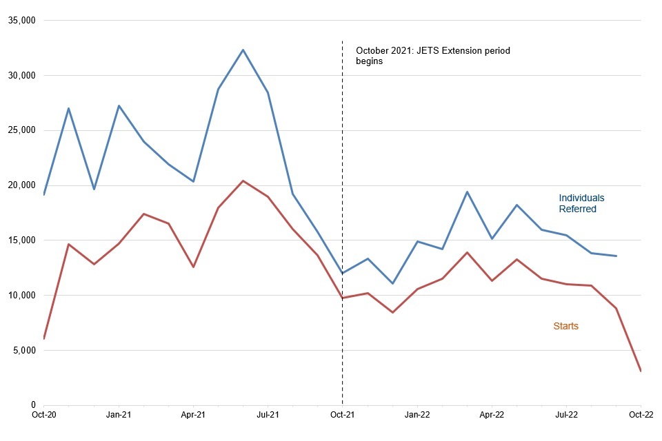
Note: Both the individuals referred and starts measures are calculated using the month in which referral or start was achieved so caution should be used in direct comparisons between both metrics.

The number of monthly individual referrals and starts peaked in June 2021 before falling away as the original 12-month JETS scheme wound down to finish in September 2021. The extension of the scheme in October 2021 for a further 12 months saw volumes rise again although not as high as previously seen levels. Individuals referred and starts decreased again in the final few months of the programme with final referrals in September 2022 and final starts in October 2022.

Across the whole lifespan of the programme, the proportion of individuals referred that started was 63%. There are several reasons why an individual may not have started on the programme. This could be because the participant found work before starting on the programme or have not worked with the provider to attend a welcome meeting within the 15 working day Service Level Agreement (SLA) period.

North East England had the highest proportion of individuals referred who started on JETS.

Proportion of all individuals referred who started on JETS broken down by area, in England and Wales, October 2020 to October 2022

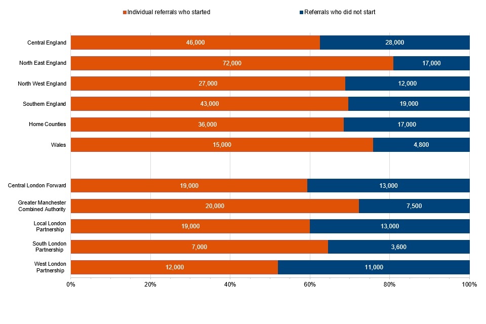
The actual number of referrals and starts varies across areas due to size. The highest proportion of individuals referred who have started was in North East England (81%) and the lowest was in West London (52%). Comparisons between regions and providers should be made with great care and the contextual differences between CPAs and LGPs should be considered.

Table: Referrals, Individuals Referred and Starts by Referral and Start month, in England and Wales, October 2020 to October 2022

Month	Referrals	Individuals Referred	Starts
Oct-20	19,000	19,000	6,100
Nov-20	28,000	27,000	15,000
Dec-20	21,000	20,000	13,000
Jan-21	30,000	27,000	15,000
Feb-21	26,000	24,000	17,000
Mar-21	24,000	22,000	17,000
Apr-21	22,000	20,000	13,000
May-21	31,000	29,000	18,000
Jun-21	35,000	32,000	20,000
Jul-21	32,000	28,000	19,000
Aug-21	22,000	19,000	16,000
Sep-21	18,000	16,000	14,000
Oct-21	13,000	12,000	9,800
Nov-21	15,000	13,000	10,000
Dec-21	12,000	11,000	8,400
Jan-22	16,000	15,000	11,000
Feb-22	15,000	14,000	12,000
Mar-22	21,000	19,000	14,000
Apr-22	17,000	15,000	11,000
May-22	20,000	18,000	13,000
Jun-22	18,000	16,000	12,000
Jul-22	17,000	15,000	11,000
Aug-22	15,000	14,000	11,000
Sep-22	15,000	14,000	8,800
Oct-22	..	..	3,100
Total	500,000	460,000	320,000

Source: DWP Provider Referral and Payment (PRaP) System

Table notes.

1. Summed values may not equal overall total due to rounding

2. “..“ denotes nil or negligible volumes.

3. Job Entry Targeted Supported (JETS) became available to all area of England and Wales in October 2020

4. Both the individuals referred and starts measures are calculated using the month in which the referral or start was achieved so caution should be used in direct comparisons between both metrics

Between January 2021 and the end of October 2022, in Scotland, there were a total of:

• 32,000 individuals referred (individuals can have multiple referrals but are only counted once)
• 23,000 starts on the scheme

Referrals to and starts on JETS peaked in February 2021 in Scotland.

Number of individuals referred to, and starting on, JETS each month between January 2021 and October 2022

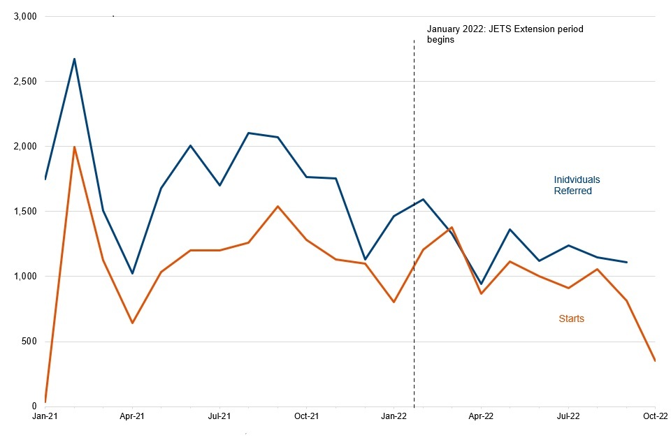
Note: Both the individuals referred and starts measures are calculated using the month in which referral or start was achieved so caution should be used in direct comparisons between both metrics.

The number of monthly individual referrals and starts peaked in February 2021, with a slow decline over the life of the programme. The extension of the scheme in January 2022 for a further 8 months saw volumes rise again although not as high as previously seen levels. Individuals referred and starts decreased again in the final few months of the programme with final referrals in September 2022 and final starts in October 2022.

Across the whole lifespan of the programme, the proportion of individuals referred that have started was 63%. There are several reasons why an individual may not have started on the programme. This could be because the participant found work before starting on the programme or have not worked with the provider to attend a welcome meeting within the 15 working day Service Level Agreement (SLA) period.

Table: Referrals, Individuals Referred and Starts by Referral and Start month, in Scotland, January 2021 to October 2022

Month	Referrals	Individuals Referred	Starts
Jan-21	1,800	1,700	40
Feb-21	2,800	2,700	2,000
Mar-21	1,800	1,500	1,100
Apr-21	1,100	1,000	640
May-21	1,800	1,700	1,000
Jun-21	2,200	2,000	1,200
Jul-21	1,900	1,700	1,200
Aug-21	2,400	2,100	1.300
Sep-21	2,300	2,100	1.500
Oct-21	2,000	1,800	1.300
Nov-21	2,000	1,800	1,100
Dec-21	1,300	1,100	1,100
Jan-22	1,700	1,500	800
Feb-22	1,800	1,600	1,200
Mar-22	1,500	1,300	1,400
Apr-22	1,100	940	870
May-22	1,600	1,400	1,100
Jun-22	1,300	1,100	1,000
Jul-22	1,400	1,200	910
Aug-22	1,400	1,100	1,100
Sep-22	1,300	1,100	810
Oct-22	..	..	350
Total	36,000	32,000	23,000

Source: DWP Provider Referral and Payment (PRaP) System

Table notes.

1. Summed values may not equal overall total due to rounding

2. “..“ denotes nil or negligible volumes.

3. Job Entry Targeted Supported (JETS) became available in Scotland from January 2021

4. Both the individuals referred and starts measures are calculated using the month in which the referral or start was achieved so caution should be used in direct comparisons between both metrics

Demographics of the JETS Scheme

In England and Wales over the lifetime of the programme of the 320,000 starts on the scheme, 42% had a recorded gender of female and 58% had a recorded gender of male.

Table: Proportion of starts on JETS by gender, in England and Wales, from October 2020 to October 2022

Volumes and proportions of starts on JETS split by recorded gender

Recorded Gender	Starts	Proportion of starts
Female	130,000	42%
Male	180,000	58%
Unknown	10	..
Total	320,000	100%

Source: DWP Provider Referral and Payment (PRaP) System, Customer Information System (CIS)

Table notes.

1. “..“ denotes nil or negligible volumes.

2. Rounding: in the table, volume of starts are rounded to the nearest 10,000. Sum of the figures may therefore not sum to 100%. These percentages are derived from unrounded figures.

3. Data for England and Wales

Across the age groups the percentage of participants who started on JETS in England and Wales was lowest for the 60+ age group at 6% and increases as the age groups decrease, to a high of 18% for the 25 to 29 age group, before a small drop to 14% for the 18-24 age group.

As noted in the introduction, Kickstart, a large-scale programme for young people, ran alongside JETS until April 2022. Therefore, it is likely that the numbers of young people starting on JETS during that period are lower than they would have been in the absence of Kickstart.

Proportion of starts on JETS by age group, in England and Wales, October 2020 to October 2022

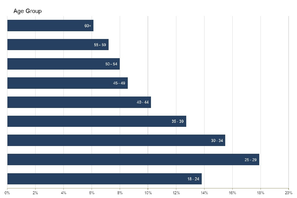
Table: Volume of Starts on JETS by gender and age, in England and Wales, from October 2020 to October 2022

Female/Male	Age	Starts
Male	Aged 16 to 17	50
Male	Aged 18 to 24	17,000
Male	Aged 25 to 29	23,000
Male	Aged 25 to 30	22,000
Male	Aged 35 to 39	19,000
Male	Aged 40 to 44	15,000
Male	Aged 45 to 49	12,000
Male	Aged 50 to 54	10,000
Male	Aged 55 to 59	9,000
Male	Aged 60+	7,600
Female	Aged 16 to 17	50
Female	Aged 18 to 24	27,000
Female	Aged 25 to 29	33,000
Female	Aged 25 to 30	27,000
Female	Aged 35 to 39	22,000
Female	Aged 40 to 44	18,000
Female	Aged 45 to 49	15,000
Female	Aged 50 to 54	15,000
Female	Aged 55 to 59	14,000
Female	Aged 60+	12,000
Unknown	All Ages	10

Source: DWP Provider Referral and Payment (PRaP) System, Customer Information System (CIS)

Table notes:

1. Summed values may not equal the overall total due to rounding applied for disclosure control.
2. Age is calculated at the point of starting on the scheme
3. Data for England and Wales

In Scotland over the lifetime of the programme of the 23,000 starts on the scheme, 35% had a recorded gender of female and 65% had a recorded gender of male.

Table: Proportion of starts on JETS by gender, in Scotland, from January 2021 to October 2022

Volumes and proportions of starts on JETS split by recorded gender

Recorded Gender	Starts	Proportion of starts
Female	8,000	35%
Male	15,000	65%
Total	23,000	100%

Source: DWP Provider Referral and Payment (PRaP) System, Customer Information System (CIS)

Table notes.

1. Rounding: in the table, volume of starts are rounded to the nearest 10,000. Sum of the figures may therefore not sum to 100%. These percentages are derived from unrounded figures.

2. Data for Scotland

Across the age groups the percentage of participants who started on JETS in Scotland was lowest for the 60+ age group at 7% and increases as the age groups decrease, to a high of 18% for the 25 to 29 age group, before a drop to 9% for the 18-24 age group.

Proportion of starts on JETS by age group, in Scotland, January 2021 to October 2022

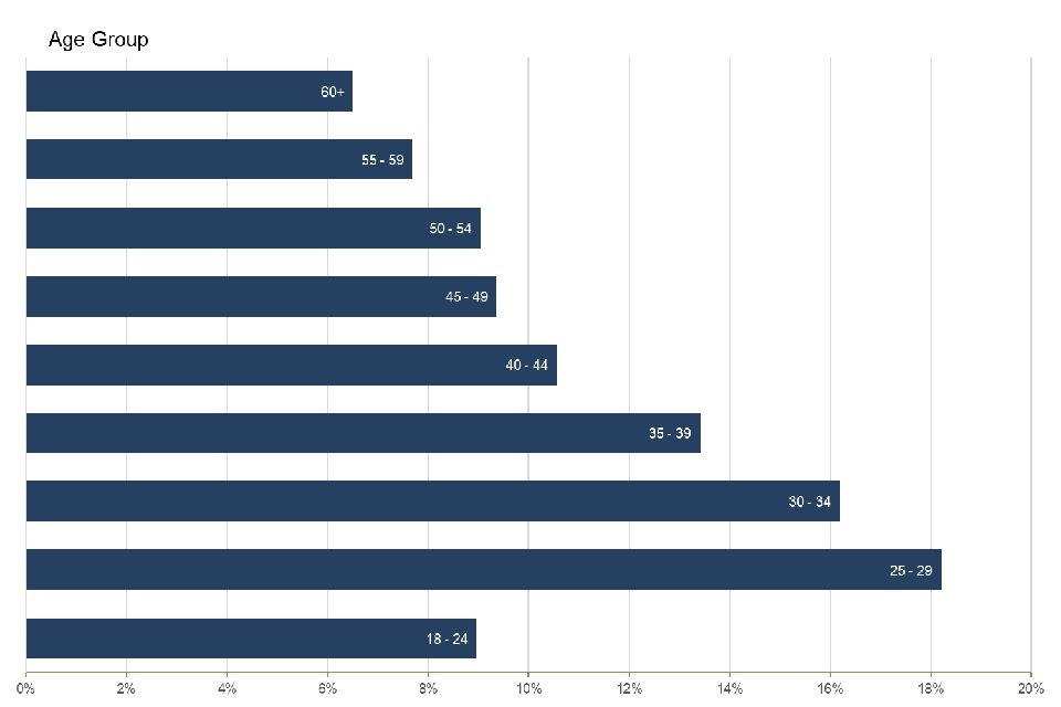
Table: Volume of Starts on JETS by gender and age, in Scotland, from October 2020 to October 2022

Female/Male	Age	Starts
Male	Aged 16 to 17	10
Male	Aged 18 to 24	1,400
Male	Aged 25 to 29	2,800
Male	Aged 25 to 30	2,300
Male	Aged 35 to 39	1,900
Male	Aged 40 to 44	1,600
Male	Aged 45 to 49	1,400
Male	Aged 50 to 54	1,400
Male	Aged 55 to 59	1,200
Male	Aged 60+	990
Female	Aged 16 to 17	10
Female	Aged 18 to 24	700
Female	Aged 25 to 29	1,400
Female	Aged 25 to 30	1,400
Female	Aged 35 to 39	1,200
Female	Aged 40 to 44	870
Female	Aged 45 to 49	800
Female	Aged 50 to 54	690
Female	Aged 55 to 59	570
Female	Aged 60+	510

Source: DWP Provider Referral and Payment (PRaP) System, Customer Information System (CIS)

Table notes:

1. Summed values may not equal the overall total due to rounding applied for disclosure control.
2. Age is calculated at the point of starting on the scheme
3. Data for Scotland

Job Outcomes on the scheme

Across the entire programme (October 2020 to July 2023), 120,000 participants reached the job outcome earnings threshold in England and Wales.

The job outcome rate in England and Wales increased as the scheme started, reaching 44% in February 2021. It then slowly decreased over the following 10 months to 33% in November 2021. It remained stable following the extension to the scheme and for the remainder of the programme.

Table: Volume and proportion of participants that have achieved a job outcome by start month, in England and Wales, from October 2020 to October 2022

Start Month	Starts	Job Outcome	Job Outcome Rate
Oct-20	6,100	2,300	38%
Nov-20	15,000	5,400	37%
Dec-20	13,000	4,900	38%
Jan-21	15,000	6,400	43%
Feb-21	17,000	7,600	44%
Mar-21	17,000	7,100	43%
Apr-21	13,000	5,300	42%
May-21	18,000	7,400	41%
Jun-21	20,000	7,800	38%
Jul-21	19,000	6,800	36%
Aug-21	16,000	5,600	35%
Sep-21	14,000	4,800	35%
Oct-21	9,800	3,400	35%
Nov-21	10,000	3,400	33%
Dec-21	8,400	2,900	34%
Jan-22	11,000	3,900	37%
Feb-22	12,000	4,200	37%
Mar-22	14,000	5,200	37%
Apr-22	11,000	4,200	37%
May-22	13,000	4,900	37%
Jun-22	12,000	4,300	37%
Jul-22	11,000	4,000	37%
Aug-22	11,000	4,000	36%
Sep-22	8,800	3,300	37%
Oct-22	3,100	1,100	34%
Total	320,000	120,000	38%

Source: DWP Provider Referral and Payment (PRaP) System

Note:

1. Summed values may not equal the overall total due to rounding applied for disclosure control.
2. These percentages are derived from unrounded figures.
3. Data for England and Wales

The highest proportion of job outcomes was within North West England

Percentage of starts achieving job outcomes on JETS, in England and Wales, by area, October 2020 to October 2022

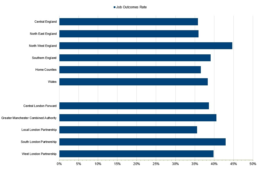
The percentage of participants who started on JETS and achieved a job outcome varies by region and was lowest for Local London, Central England, and North East England at 36% and highest for North West England at 45%.

Table: Volumes and proportion of referrals, individual referrals, starts and job outcomes, by Contract Package Area, in England and Wales: October 2020 to October 2022

Area	Referrals	Individuals Referred	Starts	Individuals who did not Start	Job Outcome	Job Outcome Rate
CPA1	81,000	74,000	46,000	28,000	17,000	36%
CPA2	94,000	89,000	72,000	17,000	26,000	36%
CPA3	43,000	39,000	27,000	12,000	12,000	45%
CPA4	68,000	62,000	43,000	19,000	17,000	39%
CPA5	58,000	53,000	36,000	17,000	13,000	37%
CPA6	22,000	20,000	15,000	4,800	5,800	38%
CLFa	35,000	32,000	19,000	13,000	7,300	39%
GMCA	30,000	27,000	20,000	7,500	8,000	41%
LLiw	35,000	32,000	19,000	13,000	6,800	36%
SLsw	11,000	10,000	7,000	3,600	2,800	43%
WLnw	26,000	23,000	12,000	11,000	4,800	40%

Source: DWP Provider Referral and Payment (PRaP) System

Notes:

1. These percentages are derived from unrounded figures.
2. Data for England and Wales

In Scotland across the entire programme (January 2021 to July 2023), 120,000 participants reached the job outcome earnings threshold.

The job outcome rate in Scotland rose in the first few months of the scheme, peaking at 45% in March 2021. The job outcome rate then slowly decreased until November 2021 (33%), rising slightly as the extension started but subsequently decreased slowly for the remainder of the programme.

Table: Volume and proportion of participants that have achieved a job outcome by start month, In Scotland, from January 2021 to October 2022

Start Month	Starts	Job Outcome	Job Outcome Rate
Jan-21	40	10	36%
Feb-21	2,000	840	42%
Mar-21	1,100	510	45%
Apr-21	640	290	44%
May-21	1,000	440	43%
Jun-21	1,200	500	42%
Jul-21	1,200	500	41%
Aug-21	1,300	460	37%
Sep-21	1,500	550	35%
Oct-21	1,300	450	35%
Nov-21	1,100	380	33%
Dec-21	1,100	380	35%
Jan-22	800	310	39%
Feb-22	1,200	430	36%
Mar-22	1,400	500	36%
Apr-22	870	310	36%
May-22	1,100	390	35%
Jun-22	1,000	330	32%
Jul-22	910	280	31%
Aug-22	1,100	320	30%
Sep-22	810	230	29%
Oct-22	350	80	24%
Total	23,000	8,500	37%

Source: DWP Provider Referral and Payment (PRaP) System

Note:

1. Summed values may not equal overall total due to rounding applied for disclosure control.
2. These percentages are derived from unrounded figures.
3. Data for Scotland

About these statistics

Key points and trends are presented using charts and commentary.

Rounding

Percentages are calculated using unrounded numbers, to the nearest whole percentage point. For these reasons, some totals may not sum to 100. The headline figures and those accompanying the graphs have been rounded as shown in the following table.

From	To	Round to nearest
0	1,000	10
1,001	10,000	100
10,001	100,000	1,000
100,001	1,000,000	10,000
1,000,001	10,000,000	100,000
10,000,001	100,000,000	1,000,000

How can this data be used?

You can use this data:

• for monitoring the overall flow of participants being referred to and starting on the JETS England & Wales Scheme and JETS Scotland Scheme, and those achieving job outcomes
• for monitoring the differences in demographics of programme participants for gender, age group and area

You cannot use this data:

• for making simple comparisons between different demographic groups (gender, age group and area) in terms of the success of the programme
• for making conclusions about the effectiveness of the programme over time or by area.

Statement of application with the Code of Practice for Statistics

The Code of Practice for Statistics (the Code) is built around 3 main concepts, or pillars:

• trustworthiness – is about having confidence in the people and organisations that publish statistics
• quality – is about using data and methods that produce statistics
• value – is about publishing statistics that support society’s needs

The following explains how we have applied the pillars of the Code in a proportionate way.

Trustworthiness

These figures have been published to provide additional information on both the JETS England & Wales and JETS Scotland Schemes. This release will give equal access to all those with an interest in them. They are published now to compliment the evaluation of JETS in England and Wales.

Quality

The data which underpins this information is taken directly from the DWP Provider Referral and Payments System, Customer information System.

The methodology and calculations have been quality assured by DWP analysts to ensure they are the best estimates using information available at the time.

Value

Producing and releasing these figures is in the public interest and provides User Organisations and the public with useful information about the JETS Scheme that they may not otherwise be able to generate or obtain.

1. See the Plan for Jobs report for a comprehensive summary of all measures adopted Plan for Jobs and employment support (parliament.uk) (accessed on 05/12/2024). ↩

2. UC-IWS and JSA are benefit regimes for individuals that are able to work but are currently not working, or working but earning very low amounts, and who are expected to take intensive action to secure work or more work. ↩

3. See the Work and Health programme Official Statistics for more information on this scheme: Work and Health Programme statistics to August 2023 - GOV.UK (www.gov.uk) (accessed on 08/04/2024). ↩

4. In Scotland and in two of the London regions, JETS was delivered through a Payment by Results Model (where part of the payments were contingent on achieving specified outcomes). ↩

5. See Work and Health Programme statistics - GOV.UK (www.gov.uk) for more information (accessed on 09/12/2024). ↩

6. See the European Social Fund statistics - (GOV.UK (www.gov.uk) for more information (accessed on 09/12/2024). ↩

7. Plan for Jobs and employment support (parliament.uk) (accessed on 11/12/2024). ↩

8. 30% had a benefit spell lasting 6 months or less, 29% had a benefit spell of between 7 and 12 months long, 20% a spell of more than 12 months but less than 24, and 21% had been 2 years or more on out-of-work or low-income benefits. ↩

9. An alternative approach to removing those individuals that started JETS in two occasions would have been to retain them in the sample and only consider their first start. We decided to remove them from the sample as the incidence was very low and the chosen approach does not require adjusting the programme cost per participant in the Cost Benefit Analysis. ↩

10. It is worth noting that non-participants could have been referred to the programme more than once. When that is the case, we use the date of the first referral to track labour market outcomes over time. It could also be that some participants were referred multiple times and their decision to start came from a second or subsequent referral. When that is the case, we use the date of the referral that led to the start. The median length between referral and start is 7 days. ↩

11. An alternative approach would have been to define treatment status using the decision to start (or not) from the first referral. While this approach has the advantage of subsequent labour market outcomes not influencing being referred and starting at later stage, the drawback is that an individual who did not start following their first referral, but started from a later referral, would be allocated to the comparison group while participating in the JETS scheme. As a sensitivity check we conducted analysis using this alternative approach and found similar employment impact estimates. ↩

12. We select a random sample due to computational limitations. For instance, when JETS started taking referrals there were over 2 million individuals claiming UC-IWS. ↩

13. Our main outcome measures employment irrespective of whether the individual is also receiving benefits. The reason is that individuals who are on Universal Credit may well remain claiming benefits after moving into employment. We also show the effect JETS had at moving participants into employment and out of unemployment related benefits in appendix figures. ↩

14. While PSM does not require the distribution of the propensity scores to be similar between participants and non-participants, a similar distribution indicates a more balanced sample before the matching. ↩

15. Other variables relating to labour market history like benefit sanctions were excluded from the analysis as they were not relevant for the population referred to JETS (only 0.2% had a benefit sanction in the past 2 years). ↩

16. Income trajectories are defined as the evolution in cumulative earnings over the 2 years prior to the referral. The inverse hyperbolic sine (IHS) transformation is frequently used to transform right-skewed variables that might contain values of 0 (like earnings) or even negative values. ↩

17. Participants are ‘on support’ if there exist at least one non-participant with a propensity score (probability to participate) that falls within the matching bandwidth defined by the matching algorithm. ↩

18. Matching with replacement allows for a single non-participant to be matched with multiple participants. ↩

19. As part of sensitivity testing different parameters are tried with little difference on the estimated results. More detail in Appendix D. ↩

20. Rubin’s B measures the absolute difference in the mean propensity scores between the treatment and the comparison group. A common accepted threshold to satisfy sample balance is 25 or below. Rubin’s R measures the ratio of the propensity score variances between the treatment and the comparison group and should lie between 0.5 and 2. A common accepted threshold for the maximum % bias is 5. ↩

21. Assessing mean differences in covariates with a t-test shows that after the matching only 7.1% of the matching variables remain statistically and significantly different at the 5% level (down from 91.6% in the unmatched sample). The proportion of matching variables with a standardised mean difference outside of the [-3%,3%] range is 64% before the matching and 0% in the matched sample. ↩

22. A lock-in effect can arise, for instance, because programme participants spend more time on training or other related activities and less time on job search than non-participants. However, the initial negative effect on employment just after programme referral could also be attributed to some individuals not starting the provision after having secured a job. While the former does not have strong implications for the estimation of longer-term impacts, the later could result in an underestimation of programme effects. ↩

23. There might be other factors that could help explain these small differences in programme effects, including differences in the characteristics of individuals starting the programme and the labour market context prevailing at the time – beyond the support available from JCP. ↩

24. While it is possible that individuals in our sample could have received other support not offered by DWP, it is not possible for us to observe this. ↩

25. These estimates are derived by conducting a separate PSM analysis for each of the sub-groups following the same procedure as for the main sample. ↩

26. The estimated difference in employment additionality between those with an out-of-work benefit spell of 7 to 12 months and those who have been on out-of-work benefits for 2 years or more is statistically significant at the 1% level. ↩

27. For a recent example, see the impact assessment of the Kickstart Scheme  (DWP, 2024): Kickstart Scheme: A Quantitative Impact Assessment - GOV.UK ↩

28. This follows a variation of the circular flow of income, where money moves back and forth between households, firms, and government. In this simplified case, firms on aggregate produce output and pay wages to individuals of equal value, who subsequently spend their wages to consume that output. Some of this money flows to the government in the form of taxes, and then flows back to households and firms through public expenditure. ↩

29. The DWP Policy Simulation Model is the main micro-simulation model used by DWP to analyse policy changes. It is based on the annual Family Resources Survey (FRS), which details benefit income streams alongside information about the circumstances of each ‘benefit unit’. ↩

30. Universal Credit Full Business Case Summary (DWP, June 2018) ↩

31. While welfare weights are derived from household income, we only observe participants’ earnings from employment. As a result, our approach assumes that participants are the sole earners in their household. ↩

32. We uprate this value for other years using the Consumer Prices Index (CPI). ↩

33. We define someone returning to employment as achieving at least £1,000 in cumulative earnings. ↩

34. While programme effects might be fully or partly sustained after year 5, there is too much uncertainty to derive meaningful estimates. ↩

35. The participant BCR can be lower when assessing costs and benefits over a longer period. This is due to costs (benefit loss and increased taxes) rising in a higher proportion than benefits (increased wages). ↩

36. In other words, we assume that 20% of the additional employment JETS created among participants would have been taken up by non-participants. ↩

37. The end dates for some benefits are not always an exact record of the end date of a claim. Often, they are inferred by a change in status between two scans of the computer systems that are typically weeks apart. In such cases the end date is assigned randomly within the range of dates between the scans. Since the dates are assigned randomly this is not expected to be a source of bias. ↩

38. A random sample is selected due to computational limitations. For instance, when JETS started taking referrals there were over 2 million individuals claiming UC-IWS. ↩

39. For instance, if there is an unobserved characteristic positively influencing participation among those referred, this is likely to be less represented among the referred non-starter group (since they have selected out on this basis) than among the non-referred group. ↩

40. We implement a more parsimonious logit model specification in the UC wider sample PSM analysis to estimate more ‘sensible’ propensity scores. If using the same set of matching variables as in the main specification (referred sample), we obtain poor pre-programme balance in the outcomes of interest. ↩