Official Statistics

Employment Data Lab analysis: The Resurgo Spear programme

Updated 31 March 2023

Applies to England, Scotland and Wales

First published: 29 November 2022
Updated: 31 March 2023

This Employment Data Lab report presents an estimate of the impact of Resurgo’s Spear Programme on the benefit, employment, and education outcomes of the programme participants. The Spear Programme is aimed at supporting young people who face barriers getting into work or education.

The results in this report have been generated using quasi-experimental techniques which introduce some uncertainty. The results should be used with a degree of caution. Further information can be found in section 7, and in an associated methodology document.

This is the first Employment Data Lab report, the layout and presentation of future versions may differ.

Headline results

Increased employment

The average participant spent between 7 and 13 more weeks in employment in the two years after starting than they would have had they not participated in the programme. This result was statistically significant.

Reduction in people classed as NEET (not in employment education or training)

The percentage of programme participants classed as NEET one year after starting the programme was between 5 and 12 percentage points less than it would have been had they not participated in the programme. This result was statistically significant.

Sustained Impact

Results show that the impacts of the intervention persist for the full two-year tracking period.

• This analysis focuses on a sub-group of 954 participants who were between the ages of 18 and 27 when they started the programme, who lived in and around London and participated between September 2015 and June 2017

• Participants were followed for two years after starting the programme (although education outcomes were available only for one year)

• Participants were compared to a comparison group of “similar” individuals to evaluate the programme

• The average number of weeks spent in employment (at two years after starting) and the percentage of the group classed as NEET (at one year after starting) were chosen as the primary outcome measures

• Other secondary outcome measures are also reported

1. What you need to know

What is the Employment Data Lab?

The Employment Data Lab is a service provided by a team of analysts at the Department for Work and Pensions (DWP). The Data Lab provides group-level benefits and employment information to organisations who have worked with people to help them into employment. The purpose is to provide these organisations with information to help them understand the impact of their programmes.

What is the Spear Programme?

The Spear Programme, created and managed by registered charity, Resurgo, aims to support young people into education or employment. The programme is targeted at individuals who are under the age of 24, not in education, employment, or training (NEET) and facing barriers to get into work. The aim of the programme is to help these individuals back into employment, education, or another favourable outcome.

The programme takes the form of a six-week intensive course with follow-up meetings over the following 12 months. The support includes coaching to overcome challenging attitudes and behaviours, and practical training such as CV writing and mock interview practice.

The Spear Programme runs in 11 centres: 7 in London and one each in Brighton, Bristol, Leeds, and Bournemouth. There are six cohorts a year per centre, and the programme has been running since January 2004, predominantly in London.

Resurgo reported that between 2015 and 2017 referrals to the Spear Programme were mainly via Jobcentre Plus (63%) followed by other referrers such as probation services, care leaving team or local authorities (22%). 9% of referrals came from a recommendation from a family or friend and 6% came from another route (including online referrals). Resurgo reported that there were drop-outs between referral and starting the project although no figures were provided.

Participant information

Of the 954 participants included in this analysis:

• 64% were male and 36% were female
• the average age was 21.0 years
• 94% were aged 18-24
• 32% were white, 29% were black, and 39% were other (including missing)
• 12% had a restricted ability to work (RATW) when they started the programme
• 58% had previously been eligible for free school meals
• 66% had previously had Special Educational Needs
• 72% were NEET on starting the programme
• 12% were employed on starting the programme

Further information about those who were (and were not) included in the analysis can be found in Appendices A and B.

Who was evaluated as part of this analysis?

Resurgo shared data on 1,824 participants who took part in the programme between September 2015 and January 2019. The analysis focussed on a subset of 954 participants who were at least 18 years old and started the programme before September 2017.

The analysis in this report

This report presents analysis on the impact of the Spear Programme by comparing employment, benefit, and education related outcomes of participants to those of a matched comparison group who did not participate. The comparison group is used to estimate the outcomes of participants had they not participated in the programme and was created using a method called propensity score matching. Further information about how the analysis was conducted can be found in the associated methodology document.

Two primary outcome measures were selected for this evaluation before the analysis was undertaken.

Primary outcome measures

The primary outcome measures for this analysis are:

• Average number of weeks spent in employment (at two years after starting), and

• The percentage of the group classed as NEET (at one year after starting).

2. Impact on labour market status

Programme participants spent more weeks in Employment

During the two years after starting the programme, the average participant spent:

• Between 7 and 13 more weeks in the Employed category than if they had not participated. This is a primary outcome measure for this evaluation

• Between 4 and 8 more weeks in the Looking for Work category than if they had not participated

• Between 2 and 5 fewer weeks in the Inactive category than if they had not participated

• Between 7 and 12 fewer weeks in the Other category than if they had not participated

These results are statistically significant.

This report uses four categories of labour market status in this analysis (see section 7 for more details).

Figure 1 and Table 1 show the impact of the programme on the average number of weeks spent in each labour market category two years after starting the intervention. The participants are compared to a comparison group used to estimate the outcomes had the participants not participated in the programme.

Figure 1: Average number of weeks spent in each labour market category in the two years after intervention start

The dark blue is the participant group, light blue is the comparison group. The end of each bar shows the central estimate, and the error bars show the upper and lower confidence values either side of the central estimate.

Table 1: Showing average number of weeks members of each group spent in each category two years after starting the programme

The impact, or difference, is shown along with an indication of statistical significance.

Category	Participant group (weeks)	Comparison group (weeks)	Impact: Central(weeks)	Impact: Lower(weeks)	Impact: Upper (weeks)	Sig.
Employed	49	39	10	7	13	yes
Looking for Work	37	31	6	4	8	yes
Inactive	9	12	-3	-5	-2	yes
Other	21	30	-9	-12	-7	yes

Note: The employed category includes those in low levels of work and receiving benefits such as Jobseekers Allowance (JSA) or Universal Credit (UC)

3. Impact on NEET status

Reduction in those classed as NEET

One year after starting the programme the percentage of participants classed as NEET was between 5 and 12 percentage points less than it would have been had they not participated.

This result was statistically significant.

This is a primary outcome measure for this evaluation

For this analysis an individual is classed as NEET at a point in time, if they are not recorded in the administrative data as being actively employed or in education or training at that time, irrespective of age.

Table 2: Showing the percentage of the participant and comparison groups classed as NEET on starting the programme and at one year after starting the programme.

The impact (difference between the two groups) at one year is shown along with an indication of statistical significance.

Time point	Participant group (%)	Comparison group (%)	Impact: Central (ppt)	Impact: Lower (ppt)	Impact: Upper (ppt)	Sig.
At start	72	72
At 12 months	40	48	-8	-12	-5	yes

The labour market transitions of those classed as NEET at start

Table 3 provides information on those who were classed as NEET when starting the programme and what they were doing one year later. The results indicate that the programme led to a decrease in people remaining NEET one year after starting, and that this was primarily driven by more people moving into employment.

The results show that of those who were classed as NEET at start:

• The number of participants who remained NEET one year later was between 4 and 10 percentage points less than had they not participated

• The number of participants in employment one year later was between 5 and 11 percentage points larger than had they not participated

• The number of participants in education one year later was between 0 and 5 percentage points larger than had they not participated

These estimates are statistically significant.

Table 3: showing the percentage of each group who transitioned from being classed as NEET at start into either employment, education or remaining as NEET one year later

These flows are presented as percentages of the total. For example, 33% of the 954 people in the matched participant group transitioned from NEET category at start to being Employed one year later. This compares to only 25% (also of 954 people) for the comparison group. The percentage point difference between these two is the impact of the programme.

Start	one year later	Participant group (%)	Comparison group (%)	Impact: Central (ppt)	Impact: Lower (ppt)	Impact: Upper (ppt)	Sig.
NEET	Employed	33	25	8	5	11	yes
NEET	Education	13	11	3	0	5	yes
NEET	NEET	33	40	-7	-10	-4	yes

Note: Figures may not sum due to rounding.

4. The impacts of the programme over time

The results show that the programme led to the following.

More classed as Employed, at one and two years

More participants being classed as Employed one and two years after starting the programme, than had they not participated.

• The increase at one year was between 7 and 14 percentage points
• The increase at two years was between 6 and 13 percentage points

More classed as Looking for Work, at one and two years

More participants being classed as Looking for Work two years after starting the programme, than had they not participated.

• The increase at one year was between 3 and 9 percentage points
• The increase at two years was between 3 and 9 percentage points

Fewer classed as Inactive, at one and two years

Fewer participants being classed as Inactive two years after starting the programme than had they not participated.

• The decrease at one year was between 2 and 6 percentage points
• The decrease at two years was between 2 and 7 percentage points

Fewer classed as Other, at one and two years

Fewer participants being classed as Other one and two years after starting the programme, than had they not participated.

• The decrease at one year was between 7 and 13 percentage points
• The decrease at two years was between 6 and 12 percentage points

These results are all statistically significant.

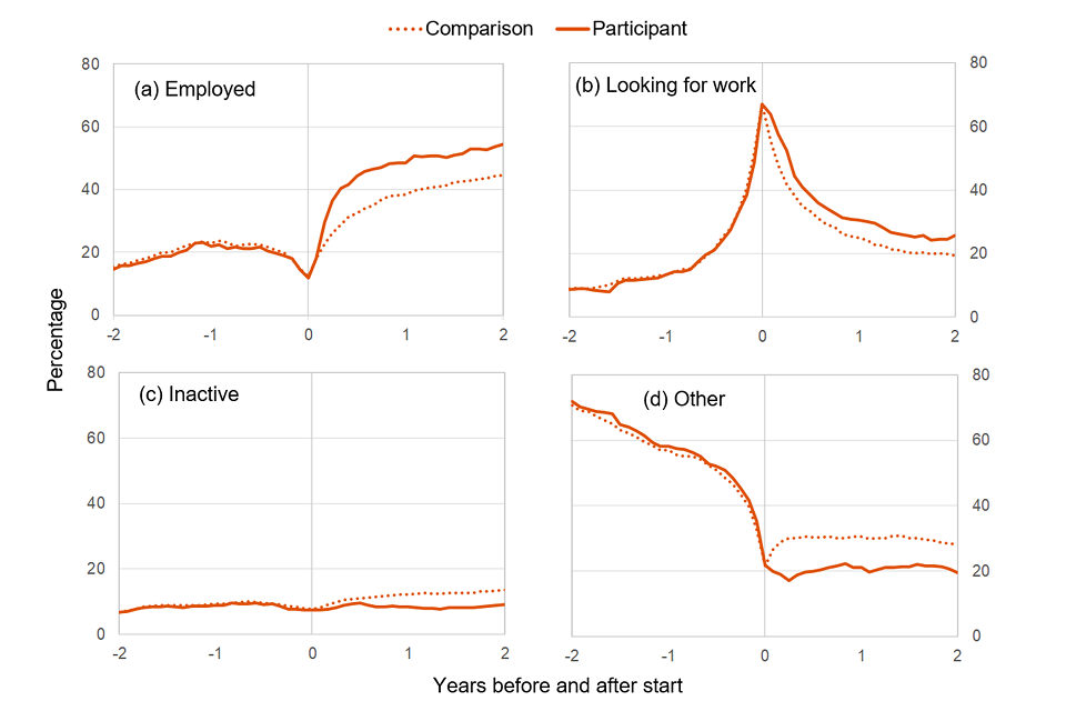
The plots in Figure 2 provide a graphical representation of how the programme impacted the percentage of participants in each labour market category: 2(a) Employed, 2(b) Looking for work, 2(c) Inactive, 2(d) Other.

The numerical figures at one and two years are presented in Table 4. A plot of the percentages of each group in each category over time can be found in Appendix F.

Figure 2: Plots showing the impact of the programme on the numbers in each labour market category over time

The impact is shown as the difference in the percentages of the participant and comparison groups in each category. The darker blue line shows the central estimate, and the shaded blue area is the 95% confidence interval.

2(a) – Employed: This plot shows that the programme had a statistically significant positive impact on the percentage of participants classed as employed that persisted for at least two years.

2(b) – Looking for work: This plot shows a smaller impact on the percentages classed as ‘looking for work’. The blue lines show that the programme led to an initial rise in this category that then fell back before staying relatively stable.

2(c) – Inactive: This plot shows that the programme led to a small but statistically significant reduction in the percentage of participants classed as ‘inactive’, that was sustained over the two-year follow-up period.

2(d) – Other: Shows that the programme led to a statistically significant and sustained reduction in the percentage of participants in the ‘other’ category.

Table 4: Showing the percentage of each group in each category at one and two years after starting the programme

The impact, or difference, is shown along with an indication of statistical significance.

Percentage of group in category	Participant group (%)	Comparison group (%)	Impact: Central (ppt)	Impact: Lower (ppt)	Impact: Upper (ppt)	Sig.
Employed (at 1 year)	49	38	10	7	14	yes
Looking for Work (at 1 year)	31	25	6	3	9	yes
Inactive (at 1 year)	8	12	-4	-6	-2	yes
Other (at 1 year)	21	31	-10	-13	-7	yes
Employed (at 2 years)	55	45	10	6	13	yes
Looking for Work (at 2 years)	26	19	6	3	9	yes
Inactive (at 2 years)	9	14	-5	-7	-2	yes
Other (at 2 years)	19	28	-9	-12	-6	yes

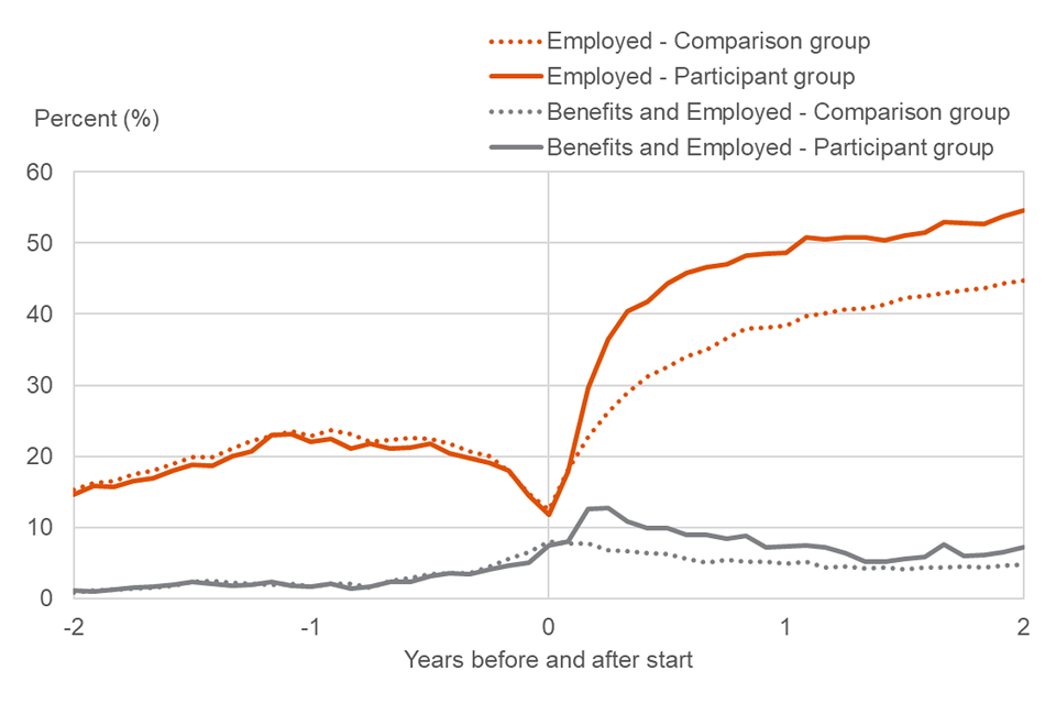
Benefits and Employment Overlap

It is important to note that the Employed category includes those in low levels of work and receiving benefits such as JSA (Jobseeker’s Allowance) or UC (Universal Credit). The plot in Figure 3 shows the percentage of each group with an employment record as well as the percentages who are employed and in receipt of “looking for work benefits”. It shows that a small percentage of the increases in employment brought about by the programme relate to low level employment where people are also in receipt of benefits.

For more information on categories see section 7.

Figure 3: Plot showing the percentages of the participant and comparison group in the Employed category and the Looking for Work and Employed category

5. How to use the results of this report?

Two primary outcome measures were chosen to assess the success of this programme. The results suggest that the programme had pronounced, positive, and statistically significant impacts on these two measures. This suggests the programme has been successful at:

• increasing employment among participants during the two years after starting the programme

• reducing the number of participants classed as NEET one year after starting the programme

A range of secondary outcome measures were also analysed in this report (see Appendix E) and can be used to learn more about the impacts of the programme. Results marked as statistically significant indicate an estimate that is unlikely to have occurred by chance (and more likely to be real). If a result is not statistically significant it does not mean that there was no impact, it just means there was insufficient evidence to verify this to the required threshold.

The estimates in this report were generated using quasi-experimental methods that can be less reliable than experimental methods such as a randomised control trial. The results should be used with a degree of caution.

The estimates relate to a programme working in a particular context. This report makes no assessment as to whether these impacts are generalisable to different contexts.

6. Resurgo in their own words

Our organisation

Resurgo exists to bring about meaningful and lasting social change in the UK. The Spear Programme is one particular expression of this, inspiring and equipping unemployed young people facing barriers to work with the skills, mindset, resources and opportunities to succeed in education or enter and sustain employment. The programme uses executive coaching techniques to help young people overcome the attitudinal and behavioural patterns that are holding them back, while equipping them with the hard skills they need to find a job.

Each Spear Centre works in partnership with local referrers to identify young people most in need of the programme. Spear Foundation then lasts for 6 weeks and is delivered by highly trained coaches with one overriding aim: getting young people ready for work or education. Spear Career provides a year of follow-on support as trainees gain greater independence and move into work or education.

Our response to the analysis

We are delighted to be the first organisation in the country to go through this evaluation with the employment data labs team, and really value the insights provided. At Resurgo, we are deeply committed to impact management, and the use of external data evaluation complements our internal processes.

The Employment Data Lab results presented here build on the growing evidence base in support of the Spear Programme, (including the ground-breaking benchmarking exercise we completed with the National Institute for Social and Economic Research using the Longitudinal Educational Outcomes Database). The results highlight the statistically significant difference the programme makes in increasing employment outcomes and reducing NEET rates for participants. The finding that the impact of our intervention is sustained for at least two years is particularly encouraging, as our current measurement practices limit our insight to 1 year after completion.

It is worth noting that this data set represents trainees who completed the programme over 5 years ago. Since then, we have continued to go through our own internal evaluation processes and have further developed the programme – for example by creating more direct employment and education opportunities for participants. It is also worth noting that this data set includes all trainees who start the programme, regardless of whether they continued to engage with us. Given our completion rate of 80%, this means that approx. 20% of the trainees included in this analysis won’t have had the full training or the years’ worth of follow-on support.

This analysis increases our confidence in the effectiveness and lasting impact of the programme, and we are grateful to the Employment Data Labs for the insight they have provided.

7. About these statistics

This report presents estimates of the impact of a programme. This is achieved by comparing the outcomes of the programme participants to a credible estimate of their outcomes had they not participated in the programme. This is often referred to as the counterfactual. In this report the counterfactual was generated using a quasi-experimental technique called propensity score matching (PSM).

This involves constructing a comparison group of individuals, who did not participate in the programme but who are matched on key characteristics that affect whether an individual takes part in the programme and the outcomes that they experience as a result of participation. Once this comparison group has been constructed the outcomes of the two groups can be compared to generate the estimate of the impact of the programme. More information about this technique and how it is used in the Data Lab can be found in the methodology report.

Categorisation

The analysis in this report is based on the labour market outcomes of the participants (and a matched comparison group) in the two years before and after starting the intervention. This report uses four categories of labour market status for the analysis:

• Employed: People who are either employed or self-employed

• Looking for Work: People who are in receipt of Jobseekers Allowance (JSA), or in the Universal Credit (UC) “intensive work search”, “light touch out of work”, “light touch in work”, or “working enough” conditionality regimes

• Inactive: People who are in receipt of inactive benefits such as Employment and Support Allowance (ESA) or in the UC “no work requirements” or “work focussed interview” conditionality regimes. Several other benefits also fall into this category, though the numbers of people on these benefits is small. See the methodology report for details

• Other: People who do not fall into the above three categories, this could include people who are in full-time education and not working or receiving benefits or those who are in custody

These categories have been designed to aid the Data Lab analysis and may not align to similar categorisations made elsewhere.

These categories are not mutually exclusive, and it is possible to be in more than one category. For example, someone working fewer than 16 hours a week may also be in receipt of JSA and would be classed as “employed” and “looking for work”.

In addition to the above categories, data on an individual’s education or training status at specific time points up to one year after starting is also used. An individual is classed as NEET at a point in time, if they do not have an active employment, education or training spell at that time, irrespective of age. More information on how benefit, employment, and education spells are generated can be found in the methodology report.

Statistical significance

The report highlights if the results are statistically significant or not. A statistically significant result is one that is unlikely to have occurred by chance because of sampling error. If a result is not statistically significant it does not mean that the intervention has no impact, it simply means that there is not enough evidence to verify this to a required threshold. In this report, unless otherwise stated, the threshold for significance is 95 per cent.

This report sometimes presents the central estimate of a result along with the upper and lower confidence values. These upper and lower values create a range that you would expect the estimate to fall within if the test was to be redone, within a certain level of confidence. This level is set at 95 per cent unless otherwise stated. The confidence intervals will typically be stated in the tables of results and be presented on graphs and plots as either error bars or shaded regions.

Limitations

The validity of the technique used in this report rests on the assumption that all the characteristics that are linked to a person’s participation in the programme and the outcome variables of interest have been sufficiently accounted for in the analysis, either explicitly or otherwise. This is a strong assumption that cannot be tested and depends on the data available and on the nature of each programme and its participants.

This is reviewed on a case-by-case basis in the Data Lab and impact evaluations are only carried out where the validity of this assumption is plausible. That said, these are quasi-experimental techniques that tend to be less robust than true experimental methods, such as a randomised control trial, and the results must be treated with a degree of caution.

Where to find out more

Read the Employment Data Lab guidance for information on how how to access the Employment Data Lab, and detail on the methodology and background.

8. Statement of compliance with the Code of Practice for Statistics

The  Code of Practice for Statistics (the Code) is built around 3 main concepts, or pillars: 

• trustworthiness – is about having confidence in the people and organisations that publish statistics

• quality – is about using data and methods that produce statistics 

• value – is about publishing statistics that support society’s needs  The following explains how we have applied the pillars of the Code in a proportionate way

Trustworthiness 

Employment Data Lab reports, such as this, are published to provide User Organisations with an estimate of the impact of their programmes that support employment. Releasing them via an ad hoc publication will give equal access to all those with an interest in them.

Quality 

The methodology used to produce the information in this report has been developed by DWP analysts in conjunction with the Institute for Employment Studies. The information is based on data from the User Organisation and Government administrative data. The calculations have been quality assured by DWP analysts to ensure they are robust.

Value 

Producing and releasing these estimates provides User Organisations and the public with useful information about employment support provision that they may not have otherwise been able to generate or obtain.

Appendix A: Exclusions from the treatment group

Resurgo shared data on 1,824 participants who took part in the programme between September 2015 and January 2019. The analysis focussed on a subset of these participants who started the programme before September 2017 and who were at least 18 years old when they started. This was to ensure that there was at least one year of follow-up educational data available and that participants were unlikely to be in compulsory full-time education one year after starting the programme.

Figure 4 shows the distribution of start dates of the programme participants.

Figure 4: Frequency plot showing the distribution of start dates for programme participants

The orange bars show the start dates of participants who were excluded as they started the programme on or after 1 September 2017.

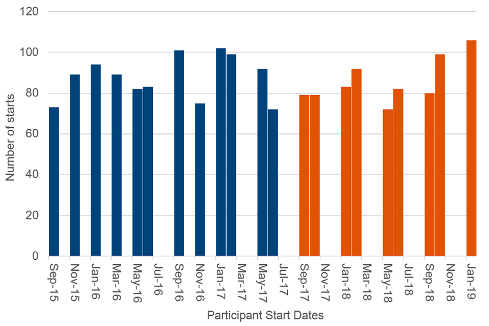
Figure 5 presents a diagram showing the numbers of participants and the stages at which they were excluded from the analysis.

The final group of 954 participants who were used in the analysis, and who could be matched to a comparator represents 91% of the participants who took part during the relevant period.

Figure 5: Numbers of the treated group that were excluded from the analysis

Appendix B: Participant group information

Table 5: Showing characteristics and benefits and employment information for the participant group

This is broken down into the “evaluated”; those who were selected for the evaluation, the “non-evaluated”; those who were excluded from the evaluation, and “all” of the treated, for whom data was available. There was an additional one participant who could not be linked to the administrative data.

Variable	Evaluated	Non-evaluated	All (with data)
Observations	954	869	1823
Age (mean years)	21.0	20.2	20.6
<18 years (%)	0	17	8
18-24 years (%)	94	79	87
25-30 years (%)	6	4	5
>30 years (%)	0	0	0
Male (%)	64	63	63
RATW at start marker set (%)	12	11	11
Partner marker set (%)	x	x	x
Partner marker missing (%)	57	72	64
Dependent children marker (%)	x	x	x
Dependent… missing (%)	19	54	36
Lone parent marker set (%)	x	x	x
Lone parent marker missing (%)	22	59	40
SEN marker set (%)	66	68	67
SEN marker missing (%)	2	5	3
FSM marker set (%)	58	62	60
FSM marker missing (%)	7	8	8
Care leaver/adopted marker (%)	x	x	x
Care leaver… missing (%)	2	5	3
Exclusion marker (%)	29	29	29
Exclusion marker missing (%)	2	5	3
Permanent exclusion marker (%)	3	x	3
Permanent … missing (%)	2	5	3
DLA/PIP marker set (%)	9	10	9
DLA/PIP at start marker set (%)	8	8	8
White ethnicity (%)	32	33	32
Black ethnicity (%)	29	26	28
Other ethnicity (%)	39	41	40
Level 1 qualification (%)	93	88	91
Level 2 qualification (%)	82	76	79
Level 3 qualification (%)	39	33	37
Level 4 qualification (%)	4	8	6
Level 5 qualification (%)	3	8	5
Level 6 qualification (%)	3	7	5
Level 7 qualification (%)	x	x	x
Level 8 qualification (%)	x	x	x
London based (%)	100	97	99
NEET at start (%)	72	66	69
Employed at start (%)	12	11	11
Looking for Work at start (%)	67	53	60
Inactive at start (%)	7	4	6
Other at start (%)	22	38	30
Number of weeks Employed in the previous two years	21	17	19
Number of weeks Looking for Work in the previous two years	20	16	18
Number of weeks Inactive in the previous two years	9	5	7
Number of weeks Other in the previous two years	59	69	63

Note: Some figures have been suppressed for disclosure control purposes.

Appendix C: Matching the comparison group

The analysis in the report uses a technique called Propensity Score Matching (PSM) to construct a comparison group of individuals that are matched on key characteristics that are linked to a person’s participation in the Programme and the outcome variables of interest. More information about this technique and how it is used in the Data Lab can be found in the methodology report.

The comparison pool was selected from the Department for Education’s (DfE) administration data and was restricted to only include individuals who were in the same age range as the participants at the time of the programme start. This group was then randomly assigned a pseudo-start date in a way that matched the distribution of participant start dates. Using the information on the individual’s location at the pseudo-start date (using NUTS (Nomenclature of Territorial Units for Statistics) level 2), this group was reduced further to ensure that the locations and percentages of the group in these locations matched the participant group. This group of 192,366, the comparison pool, was then used in the matching process.

The matching estimator used to generate the impact estimates presented in this report was nearest neighbour matching using 100 nearest neighbours and a bandwidth of 0.01. Nearest neighbour matching involves running through each participant and matching them with the closest eligible individuals from the comparison pool, determined by closeness of the propensity scores. The sensitivity of the impact estimates to the choice of matching estimator was tested and the result of this are presented in Appendix D. Further information about matching estimators can be found in the methodology and literature review documents.

Table 6 shows the variables used in the matching process and the mean values of these variables both before and after matching. The table shows that before matching the participant and comparison groups are not well matched, or balanced, shown by sizeable differences in the mean values. After matching the mean values of the participant and comparison groups are much closer. The percent bias and p-value columns provide information on how big the residual difference is and if this difference is statistically significant. Ideally one would like the percent biases to be small (below 5%) and there to be no statistically significant differences i.e., p-values above 0.05 (the 95 percent confidence level threshold).

Table 7 also presents some summary statistics that relate to how well matched the participant and comparison groups are for each of the sensitivity runs. It shows values for Rubin’s B, Rubin’s R and the maximum and median percent biases, all of which meet commonly accepted thresholds for the selected approach (see the methodology report for more details). The table also shows there were only 19 participants (2 percent) who were off support, a sufficiently small percentage so as not to raise concerns about the representativeness of the results.

Table 6 Showing mean value of each control variable, for each group, before and after matching

The residual percent bias and p-value (after matching) are also shown.

Variable	un-matched comparison group	un-matched participant group	matched comparison group	matched participant group	percent bias	p value
c_month_m_6	11	11	9	11	5.06	0.25
fsm_new	30	57	61	58	-4.80	0.31
c_month_m_12	17	16	15	17	4.64	0.30
c_month_m_9	14	14	12	14	4.54	0.31
exclusion	12	28	30	29	-4.40	0.41
wp_hist	x	6	7	6	-4.13	0.48
binary_jsahist	10	55	56	54	-3.89	0.48
o_month_m_15	46	62	60	62	3.88	0.39
binary_emphist	74	51	53	51	-3.85	0.43
c_month_m_15	18	18	17	18	3.76	0.41
o_month_m_18	48	65	63	65	3.73	0.41
o_month_m_3	38	46	44	45	3.69	0.42
c_month_m_18	19	19	18	19	3.66	0.42
l_month_m_18	x	11	11	11	-3.48	0.55
c_month_m_24	26	29	28	29	3.45	0.46
i_month_m_3	4	8	9	8	-3.44	0.52
w_month_m_15	49	21	22	21	-3.29	0.43
c_month_m_21	22	24	23	24	3.26	0.48
o_month_m_21	51	69	67	69	3.09	0.49
f_ratw_start	4	12	12	12	0.68	0.90
c_month_m_3	11	11	10	11	2.95	0.51
f_miss_loneparent	84	22	21	22	2.88	0.55
f_ethnicity_2_black	16	29	30	29	-2.87	0.57
f_miss_children	82	19	18	19	2.83	0.54
l_month_m_21	3	9	9	8	-2.82	0.62
w_month_m_18	47	19	20	19	-2.66	0.51
snc_hst_flg	x	18	18	18	-2.66	0.66
binary_uc_iwshist	x	30	29	30	2.64	0.67
binary_icahist	x	x	x	x	2.57	0.61
sen_new	28	65	67	66	-2.47	0.60
level_2_start	89	80	81	82	2.46	0.62
o_month_m_24	53	72	71	72	2.37	0.59
o_month_m_12	44	58	57	58	2.34	0.61
o_month_m_6	40	53	51	52	2.29	0.62
f_age	22.5	21.0	21.1	21.0	-2.19	0.57
c_start	10	10	10	10	2.14	0.64
c_week_m1	10	10	10	10	2.14	0.64
i_month_m_6	4	9	10	9	-2.11	0.70
f_age_sq	513.2	445.0	447.3	445.1	-2.08	0.58
binary_ishist	3	5	6	6	-2.03	0.70
w_month_m_21	44	16	17	17	-2.02	0.61
w_month_m_3	56	19	20	19	-1.99	0.62
i_month_m_9	4	9	10	9	-1.99	0.72
level_3_start	64	39	38	39	1.92	0.68
binary_uc_misshist	x	x	x	x	-1.90	0.75
w_month_m_12	51	22	23	22	-1.89	0.65
i_week_m1	4	7	8	7	-1.87	0.72
intervention_year	2016.2	2016.2	2016.2	2016.2	-1.83	0.69
l_month_m_15	x	12	12	12	-1.82	0.76
f_ethnicity_2_white	34	31	31	32	1.77	0.70
w_week_m1	57	12	13	12	-1.71	0.64
level_4_start	27	4	5	4	-1.67	0.55
i_start	4	7	8	7	-1.65	0.75
o_month_m_9	42	57	55	56	1.64	0.72
o_week_m1	37	25	24	25	1.63	0.70
a_month_m_3	9	13	12	13	1.58	0.74
missing_fsm_new	23	9	7	7	1.53	0.64
binary_uc_ltoowhist	x	x	x	x	-1.52	0.80
w_start	57	12	12	12	-1.49	0.68
i_month_m_18	4	8	9	9	-1.47	0.79
w_month_m_6	54	22	22	22	-1.46	0.73
i_month_m_15	4	8	9	9	-1.40	0.80
w_month_m_24	42	15	15	15	-1.40	0.71
binary_esahist	4	11	11	11	-1.37	0.81
l_month_m_6	x	21	21	21	-1.36	0.82
dlapip_start	3	8	7	8	1.35	0.81
h_month_m_18	19	6	7	6	-1.33	0.71
a_month_m_15	12	26	26	27	1.31	0.80
h_month_m_21	19	7	8	7	-1.31	0.72
f_loneparent	3	x	x	x	-1.27	0.76
i_month_m_12	4	9	9	9	-1.25	0.82
binary_uc_eehist	x	x	x	x	-1.20	0.83
binary_dlapiphist	3	8	8	9	1.12	0.84
a_month_m_18	10	24	23	24	1.12	0.83
l_week_m1	3	64	64	63	-1.12	0.86
intervention_month	5.6	5.6	5.7	5.6	-1.09	0.81
wp_start	x	x	3	x	-1.04	0.86
f_partner	x	x	x	x	1.03	0.83
a_week_m1	9	7	8	7	-1.03	0.81
l_month_m_3	x	32	33	33	-0.98	0.87
a_month_m_12	13	29	29	29	0.98	0.85
f_children	3	x	x	x	-0.96	0.82
l_month_m_24	3	9	9	9	-0.94	0.87
level_5_start	25	3	3	3	-0.93	0.71
level_6_start	24	3	3	3	-0.91	0.70
o_start	37	21	21	22	0.85	0.84
f_miss_partner	90	57	56	57	0.77	0.89
permanent	x	3	3	3	0.75	0.89
a_month_m_6	9	17	16	17	0.74	0.89
level_1_start	94	91	93	93	0.73	0.87
h_month_m_24	19	7	8	7	-0.73	0.84
f_ethnicity_2_other	51	40	39	39	0.71	0.88
h_month_m_15	20	7	8	7	-0.59	0.87
l_month_m_9	x	15	15	15	-0.56	0.93
i_month_m_21	4	8	8	8	-0.55	0.92
h_month_m_6	20	6	5	6	0.54	0.87
i_month_m_24	3	6	7	7	-0.49	0.93
a_month_m_21	12	31	31	32	0.48	0.93
h_month_m_12	20	7	7	7	-0.38	0.91
w_month_m_9	52	22	22	22	-0.35	0.93
h_month_m_3	21	4	4	4	0.31	0.91
missing_exclusion	x	3	x	x	0.27	0.95
missing_permanent	x	3	x	x	0.27	0.95
missing_sen_new	x	3	x	x	0.27	0.95
l_start	3	68	67	67	-0.27	0.97
missing_cla_adopt	x	3	x	x	0.27	0.95
a_month_m_24	13	33	34	34	-0.26	0.96
binary_uc_ltiwhist	x	x	x	x	-0.26	0.96
h_week_m1	21	x	3	3	-0.24	0.92
a_start	10	7	7	7	-0.20	0.96
f_sex	50	64	64	64	-0.20	0.96
a_month_m_9	11	23	23	23	0.17	0.97
l_month_m_12	x	13	13	13	-0.16	0.98
h_start	21	x	x	x	-0.10	0.96
binary_uc_wfihist	x	x	x	x	-0.08	0.99
binary_sahist	6	x	x	x	-0.04	0.99
h_month_m_9	20	6	6	6	0.00	1.00
binary_bbhist	x	x	x	x	x	x
binary_bsphist	x	x	x	x	x	x
binary_ibhist	x	x	x	x	x	x
binary_pibhist	x	x	x	x	x	x
binary_sdahist	x	x	x	x	x	x
binary_uc_wprephist	x	x	x	x	x	x
binary_wbhist	x	x	x	x	x	x
cla_adopt	x	x	x	x	x	x
level_7_start	x	x	x	x	x	x
level_8_start	x	x	x	x	x	x
missing_level_1_start	x	x	x	x	x	x

Note: Some figures have been suppressed for disclosure control purposes.

The definition of the matching variables can be found in the methodology document.

Appendix D: Sensitivity Analysis

Analysis was carried out to test the sensitivity of the impact estimates to changes in the matching algorithm. Table 7 presents the outputs of the selected method alongside four other test runs where a different matching estimator or bandwidth was used. The table shows that alternative methods resulted in matched comparison groups with similar balance scores and the impact estimates were consistent with the selected approach.

For more information on propensity score matching methods see the literature review document.

Table 7: Sensitivity of Results to changes in the matching algorithm

Run:	Selected approach	Test 1	Test 2	Test 3	Test 4
Matching estimator	Nearest Neighbour	Nearest Neighbour	Kernel	Kernel	Radius
Detail	N=100	N=100	Normal	Epan
bandwidth/calliper	0.01	0.001	0.001	0.001	0.001
Rubin’s B	15.94	17.29	21.87	19.21	18.78
Rubin’s R	0.90	0.94	0.77	0.91	0.88
Max % bias	5.06	5.74	7.37	6.13	5.82
Median % bias	1.49	1.47	1.54	1.60	1.57
No. on support	954 (98%)	933 (96%)	957 (98%)	933 (96%)	933 (96%)
No. off support	19 (2%)	40 (4%)	16 (2%)	40 (4%)	40 (4%)
Impact at 1 year: Employed (no. of weeks)	4.91	5.00	4.49	4.74	4.63
Impact at 1 year: Standard error	0.67	0.69	0.71	0.71	0.70
Impact at 2 years: Employed (no. of weeks).	10.01	10.26	9.23	9.82	9.63
Impact at 2 years: Standard error	1.29	1.33	1.36	1.36	1.35
Impact at 1 year: Looking for work (no. of weeks)	3.39	3.66	3.42	3.72	3.68
Impact at 1 year: Standard error	0.65	0.67	0.63	0.64	0.64
Impact at 2 years: Looking for work (no. of weeks)	6.18	6.71	6.19	6.78	6.77
Impact at 2 years: Standard error	1.15	1.18	1.11	1.13	1.13
Impact at 1 year: Inactive (no. of weeks)	-1.14	-1.12	-0.86	-1.07	-1.01
Impact at 1 year: Standard error	0.49	0.51	0.45	0.46	0.46
Impact at 2 years: Inactive (no. of weeks).	-3.48	-3.47	-2.96	-3.34	-3.26
Impact at 2 years: Standard error	0.93	0.96	0.86	0.87	0.86
Impact at 1 year: Other (no. of weeks)	-4.91	-5.27	-4.81	-5.09	-5.01
Impact at 1 year: Standard error	0.60	0.63	0.63	0.62	0.62
Impact at 2 years: Other (no. of weeks)	-9.44	-10.11	-9.16	-9.81	-9.72
Impact at 2 years: Standard error	1.10	1.15	1.13	1.13	1.12
Impact % NEET at 1 year	-8.28	-8.55	-7.45	-8.63	-8.24
Standard error	1.75	1.80	1.74	1.75	1.75

Appendix E: Table of results

Table 8 Showing the full list of generated results

Outcome measure	Participant group	Comparison group	Impact: central	Impact: lower	Impact: upper	p-value
no. weeks at 1 year - employed	21.4	16.4	4.9	3.6	6.2	0.00
no. weeks at 1 year – looking for work	22.7	19.3	3.4	2.1	4.7	0.00
no. weeks at 1 year - inactive	4.4	5.6	-1.1	-2.1	-0.2	0.02
no. weeks at 1 year - other	10.0	14.9	-4.9	-6.1	-3.7	0.00
no. weeks at 2 years - employed	48.7	38.7	10.0	7.5	12.6	0.00
no. weeks at 2 years - looking for work	36.7	30.5	6.2	3.9	8.4	0.00
no. weeks at 2 years – inactive	8.8	12.2	-3.5	-5.3	-1.7	0.00
no. weeks at 2 years - other	20.5	29.9	-9.4	-11.6	-7.3	0.00
% at 1 year - employed	48.6	38.4	10.3	6.8	13.7	0.00
% at 2 years -employed	54.5	44.7	9.8	6.3	13.3	0.00
% at 1 year - looking for work	30.6	24.9	5.7	2.6	8.7	0.00
% at 2 years - looking for work	25.6	19.4	6.1	3.2	9.0	0.00
% at 1 year - inactive	8.4	12.2	-3.8	-5.8	-1.8	0.00
% at 2 years -inactive	9.0	13.5	-4.5	-6.6	-2.4	0.00
% at 1 year - other	21.0	30.5	-9.5	-12.5	-6.6	0.00
% at 2 years - other	19.5	28.2	-8.7	-11.6	-5.8	0.00
% in education at 3 months	20.4	20.3	0.1	-2.8	3.0	0.94
% in education at 6 months	23.2	20.0	3.2	0.2	6.2	0.03
% in education at 9 months	23.6	21.4	2.2	-0.8	5.2	0.15
% in education at 12 months	23.9	21.2	2.7	-0.3	5.7	0.08
% neet at 3 months	49.7	58.3	-8.6	-12.1	-5.1	0.00
% neet at 6 months	43.4	53.7	-10.3	-13.8	-6.8	0.00
% neet at 9 months	41.2	49.2	-8.0	-11.4	-4.5	0.00
% neet at 12 months	39.9	48.2	-8.3	-11.7	-4.9	0.00
% work (start) to work (1 yr)	8.2	8.5	-0.3	-2.3	-1.7	0.75
% work (start) to education (1 yr)	3.0	x	0.6	-0.6	1.8	0.36
% work (start) to NEET (1 yr)	x	3.2	-0.2	-1.4	1.0	0.72
% education (start) to work (1 yr)	9.5	6.3	3.3	1.2	5.3	0.00
% education (start) to education (1 yr)	8.6	8.9	-0.3	-2.4	1.8	0.81
% education (start) to NEET (1 yr)	4.4	5.3	-0.9	-2.4	0.6	0.23
% NEET (start) to work (1 yr)	32.8	24.8	8.0	4.9	11.2	0.00
% NEET (start) to education (1 yr)	13.4	10.7	2.7	0.4	5.0	0.02
% NEET (start) to NEET (1 yr)	32.9	40.1	-7.2	-10.5	-3.9	0.00
% at 1 year in work only	40.0	32.5	7.6	4.2	11.0	0.00
% at 2 years in work only	45.9	39.0	7.0	3.5	10.4	0.00
% at 1 year in looking for work only	23.3	19.9	3.4	0.6	6.2	0.02
% at 2 years in looking for work only	18.3	14.6	3.7	1.2	6.3	0.00
% at 1 year in inactive only	7.1	11.1	-4.0	-5.9	-2.1	0.00
% at 2 years in inactive only	7.7	12.5	-4.8	-6.8	-2.9	0.00
% at 1 year in other	21.0	30.5	-9.5	-12.5	-6.6	0.00
% at 2 years in other	19.5	28.2	-8.7	-11.6	-5.8	0.00
% at 1 year in looking for work & work	7.3	4.9	2.4	0.7	4.1	0.01
% at 2 years in looking for work & work	7.2	4.7	2.5	0.8	4.2	0.00
% at 1 year in inactive and work	x	x	0.3	-0.5	1.1	0.44
% at 2 years in inactive and work	x	x	0.4	-0.4	1.2	0.36
% at 1 year in looking for work & inactive	x	x	-0.1	-0.1	0.0	0.00
% at 2 years in looking for work & inactive	x	x	-0.1	-0.1	0.0	0.01

Note: Some figures have been suppressed for disclosure control purposes.

Appendix F: Labour market category percentages before and after programme start

Figure 6: Plots showing the percentages of the participant (solid orange) and comparison group (dotted orange) in each category

Appendix G: Glossary of Terms

Term	Definition
Common support/On Support/Off support	Once propensity scores have been assigned for each observation, the overlap of propensity scores between the participants and comparison group is called ‘common support’. Those who fall in the overlap are referred to as ‘on support’, those who do not fall into the overlap are ‘off support’.
Comparison group	Carefully selected subset of the comparison pool, selected to have outcomes as similar as possible, to act as a counterfactual.
DfE	Department For Education
DLA	Disability Living Allowance
DWP	The Department for Work and Pensions
ESA	Employment and Support Allowance
FSM	Free School Meals
JSA	Jobseeker’s Allowance
NEET	Not in Employment, Education or Training
Participant group	The people who took part in the programme being evaluated.
PIP	Personal Independence Payment
Programme	The employment support provision under investigation.
Pseudo-start date	Dates assigned to the comparison pool in lieu of the real programme start dates of the participant group.
PSM	Propensity Score Matching
Quasi-Experimental	An experimental technique that looks to establish a cause and effect relationship between two variables, where the assignment to the participant or comparison group is not random.
Rubin’s B & R	A test used to evaluate the matching in PSM
SEN	Special Educational Needs
Statistically significant	Describes a result where the likelihood of observing that result by chance, where there is no genuine underlying difference, is less than a set threshold. In the Data Lab reports, this is set at 5 per cent.
UC	Universal Credit
User Organisation	The organisation using the employment data lab service.

Feedback

We welcome feedback.

We are committed to improving the official statistics we publish. We want to encourage and promote user engagement, so we can improve our statistical outputs. We would welcome any views you have using the following contact information.

Media enquiries

Contact the DWP press office.

Statistical contacts

L Barclay, J Crowe, J Freestone: employment.datalab@dwp.gov.uk