Employment Data Lab: methodology report
Updated 9 July 2026

© Crown copyright 2026
This publication is licensed under the terms of the Open Government Licence v3.0 except where otherwise stated. To view this licence, visit nationalarchives.gov.uk/doc/open-government-licence/version/3 or write to the Information Policy Team, The National Archives, Kew, London TW9 4DU, or email: psi@nationalarchives.gov.uk.
Where we have identified any third party copyright information you will need to obtain permission from the copyright holders concerned.
This publication is available at https://www.gov.uk/government/publications/employment-data-lab-information-and-guidance/employment-data-lab-methodology-report
Summary
This document provides a detailed description of the approach used to produce the Employment Data Lab evaluation reports. This document covers the full process with a focus on the data sources and matching methods used to estimate the impact of employment support programmes.
Further detail about the evaluations can be found in the reports themselves.
General information about the service and how to access it can be found in the Employment Data Lab webpages.
The methodology outlined in this document builds on the literature review and methodological background document.
Authors
Luke Barclay, Adam Raine, Sarah Hunt, William Bowers, James Crowe and Joe Freestone (analysts at, or formally at, the Department for Work and Pensions).
Dr Helen Gray is Chief Economist at Learning and Work Institute and formerly Principal Research Economist at the Institute for Employment Studies.
Acknowledgements
Thanks are due to the many colleagues within the Department for Work and Pensions and outside to the external Advisory Board, who have contributed to this report and the development of the Employment Data Lab service.
Glossary of terms
| Term | Definition |
|---|---|
| CIA | Conditional Independence Assumption |
| Comparison group | Carefully selected subset of the comparison pool, selected to have characteristics as similar as possible, to act as a counterfactual |
| Comparison pool | Individuals, with similar characteristics to those who participated, used to approximate participant outcomes had there been no programme. A matched comparison group is selected (using matching methods) from the broader comparison pool. |
| Counterfactual | Estimate of the outcomes that participants would have attained if the programme had not been introduced. |
| DfE | Department for Education |
| DOB | Date of Birth |
| DPIA | Data Protection Impact Assessment |
| DWP | Department for Work and Pensions |
| ESA | Employment Support Allowance |
| GDPR | General Data Protection Regulation |
| HESA | Higher Education Statistics Agency |
| HMRC | HM Revenue and Customs |
| ILR | Individualised Learner Records data |
| JSA | Jobseeker’s Allowance |
| Matching methods | Method used to select the comparison group from the comparison pool. |
| MSB | Mean Standardised Bias |
| NEET | Not in Employment, Education or Training |
| NINO | National Insurance Number |
| NPD | National Pupil Database |
| Participant group | The group of individuals who participated in the programme being evaluated. |
| PD | Personal Data |
| Programme or intervention | The employment support provision being evaluated. |
| Propensity score | The probability that an individual with a given set of characteristics has some chosen attribute, for example, participates in an intervention. |
| PSM | Propensity Score Matching |
| Statistically significant | Describes a result where the likelihood of observing that result by chance, where there is no genuine underlying difference, is less than a set threshold. In the Data Lab reports this is set at 5 per cent. This means that there is a 5 in 100 chance that a difference is observed when no difference exists. |
| UC | Universal Credit |
| User Organisation | The organisation using the Employment Data Lab service. |
Chapter 1 Introduction
1.1 About the DWP Employment Data Lab
1.1.1 Aims
The DWP Employment Data Lab was set up by the Department for Work and Pensions (DWP) to use existing datasets to evaluate the impact of employment-related interventions delivered by external User Organisations, such as local authorities, charities, and private sector providers. Such organisations cannot often carry out these evaluations without support from DWP as they are unable to access the necessary administrative data.
The aim of the service is to produce robust evidence on the impact of a wide range of different types of interventions where participation is on a voluntary basis. By improving the evidence base, the Data Lab seeks to improve the effectiveness of employment programmes run both by DWP and by third parties. The Data Lab works by User Organisations sharing information about the participants of their programme with the Data Lab team at DWP. This is then analysed and where possible the impact of their programme is estimated and shared back.
The initial objective of the Data Lab was to identify and implement a methodological approach suited to producing robust[footnote 1] and defensible estimates of the causal impact of a wide range of employment-related interventions. To do this in a timely manner it has been necessary to develop a standardised approach to the evaluations. It is this approach that is outlined in this document.
The longer-term aim is to continue developing the Data Lab over time. This could potentially include:
- incorporating additional sources of data
- making improvements to the software used
- reflecting developments in evaluation methods
- using other evaluation techniques to allow a wider range of interventions to be evaluated
1.2 Estimating impact
To estimate the impact of any intervention it is necessary to form a credible estimate of the outcomes that those subject to the intervention (or those eligible to participate, if participation cannot be observed) would have attained if the programme had not been introduced. This estimate of outcomes is known as the counterfactual.
Provided the approach to estimating counterfactual outcomes is sound, any difference between counterfactual and observed participants outcomes can be attributed to the impact of the intervention.
For the estimate of the counterfactual to reflect likely outcomes for participants if they had not received the intervention, it is necessary to adjust for any changes in outcomes over time that might have occurred even without the intervention, for example, if a macroeconomic shock, or the introduction of other labour market programmes, made it easier, or harder, to find a job[footnote 2].
The Data Lab uses matching methods to estimate counterfactual outcomes. This involves identifying a comparison pool of individuals likely to experience similar outcomes to participants in the intervention. From this pool of potential comparators, the subset which are most similar to participants are identified. Outcomes for these matched comparators are then deducted from outcomes for participants to form an estimate of the impact of the intervention. Chapter 4 provides a more detailed description of the methods used by the Data Lab.
These matching methods rely on the use of rich and detailed data such that the full range of factors likely to affect whether an individual participates in a programme can be allowed for. The administrative data that the Data Lab team have access to are well suited to this task and are discussed in Chapter 2. How the data are used, and the associated limitations and assumptions are discussed in Chapter 4.
The primary aim of the Data Lab is to provide estimates of the impact of employment interventions. In some cases this may not be possible, perhaps due to sample size issues or problems in identifying a suitable comparison group. Where it is decided that an impact evaluation is not appropriate the team will provide a descriptive analysis, detailing the characteristics, benefit and employment histories and outcomes of programme participants without an assessment of causal impact.
1.3 Methodological background
The methodology is based on the recommendations made in an earlier literature review, which considered a range of different evaluation methods which might potentially be used by the Employment Data Lab team. As well as outlining the main findings from relevant literature, including past evaluations of active labour market programmes and technical papers on the causal identification of impact, the literature review sets out a proposed methodology for use in the Employment Data Lab. The literature review provides detailed background information on the reasons why the approach set out in the current report was chosen.
The Employment Data Lab team implemented the recommendations set out in the literature review and this methodology report provides a description of the methods used currently to produce outputs. Future versions of the methodology report will be released as the approach is refined and methods expanded to suit a wider range of intervention types.
1.4 An overview of processes
This section lays out the steps taken by the Data Lab team when producing an evaluation report. Each of the steps is described in detail in the chapters which follow.
-
Decision on the programme’s suitability for the data lab: After initial contact, the nature of the programme and its objectives are discussed with the User Organisation and the programme’s suitability for the Data Lab service is assessed by the Data Lab team. See section 3.2.
-
Data Supply from User organisation: If the programme is deemed suitable, identifiable participant information must be supplied by the User Organisation (names, addresses, etc.). See section 3.3
-
Data linking: Once the participant data are received by the Data Lab team, the participants must be found within DWP’s administrative datasets. See section 3.4.
-
Linking to other administrative data: Having located the participants within the DWP administrative datasets, further data from other government department’s administrative datasets is linked for use in the analysis. See section 3.5.1
-
Descriptive analysis: Descriptive statistics are produced. See section 4.1
-
Decision on approach to analysis: The programme and the available data are reviewed to decide if an impact evaluation using matching methods is appropriate or not. See section 4.2.2
-
Create a comparison pool: A group of potentially eligible people who did not participate in the User Organisation’s programme is selected and decisions around a reference date for the analysis are made. See section 3.6
-
Estimate propensity scores and match: Matching methods are used to create a “matched comparison group” from the larger comparison pool. See sections 4.2.5 and 4.2.6.
-
Assess “balance”: Once matched, an assessment is made about how well matched the participant and comparison groups are, and a decision is made as to if they are sufficiently well matched to proceed. See section 4.2.7.
-
Estimate impact: The impact of the programme is estimated by comparing the outcomes of the participant and comparison groups. See section 4.2.8.
-
Report impact and/or outcomes: The results are compiled into a report and published on gov.uk. See section 4.3.
-
Archiving and data destruction: See section 2.1.2.
Chapter 2 Data sources
Situated within DWP, the Employment Data Lab has access to a wide range of administrative data gathered by DWP and other Government Departments, for the purposes of carrying out Government functions. Such data tend to have very wide coverage (close to population level) and can span long time periods of several decades. This makes it well suited to the matching methods used in the Data Lab. The service currently uses data from 4 main sources:
-
data from User Organisations, which includes identifiable information about participants and the date they started the intervention, as well as general information about the intervention
-
DWP administrative datasets, which provide details of spells on DWP benefits and employment programmes as well as characteristics of DWP customers
-
HM Revenue and Customs (HMRC) Tax System, which provides details of employment spells
-
Department for Education (DfE) administrative datasets, which provides details on time spent in education and training, qualifications obtained and other associated characteristics such as eligibility for free school meals or special educational needs status. These datasets are often referred to as the Longitudinal Education Outcomes (LEO) datasets.
2.1 Data from User Organisations
The service relies on User Organisations sharing information about the intervention under consideration. Crucially this must include personal data (PD) for the participants, so that they can be located and linked to DWP’s datasets. Details of the intervention, its aims and how people are selected, as well as information about the lawful basis for the transfer and metadata for the transferred files must also be provided. Further details about this information are provided below.
2.1.1 The Data:
User Organisations must supply information on three aspects of the transfer: general intervention details, participant details, and file metadata.
The intervention details are used to help determine the approach to the analysis and must consist of the following:
- description of the intervention including desired outcomes or success criteria
- primary eligibility criteria
- other eligibility or selection criteria
- timeframe of when we should expect to see the impacts of the programme. This helps to determine when the right time is to conduct the evaluation
The participant details are used to match and link[footnote 3] participants to DWP’s data sets. They must also include information about the individual’s participation in the intervention, in particular a start date (and end date where appropriate). If any other sub-analysis is required, such as comparing different types of intervention, appropriate identifiers must also be included. The PD required for matching would typically include the following:
- First name
- Surname
- Date of Birth
- Postcode (and other address lines if available)
Other variables such as gender and middle names or initials can also be used to help with matching and verification. If a participant’s National Insurance Number (NINO) is available this will substantially increase the chances of linking.
DWP also asks for file metadata to be supplied alongside the data file. These data should include information on the number and size of files being transferred, a list of the variables included, and the format of the files. The file metadata are used on receipt of the data at DWP as part of standard security checks.
2.1.2 Data retention
The identifying data received by DWP will be stored in a non-persistent area of DWP’s servers and deleted 90 days after processing.
After the initial linking the data is “pseudonymised[footnote 4]”, or stripped of explicit personal identifiers, for use by the Data Lab team for analysis. This data will typically be kept for 24 months unless otherwise agreed with the User Organisation.
2.1.3 Lawfulness
It is the responsibility of the User Organisation to recognise and understand their responsibilities under GDPR (General Data Protection Regulation) and the Data Protection Act 2018 in relation to the data that they are sharing. The User Organisation must acknowledge this and declare the lawful basis (and where appropriate the legal powers) on which they are relying for the data share before any transfer of data can be made. Organisations are also responsible for carrying out their own Data Protection Impact Assessment.
2.2 DWP administrative datasets
DWP collects data to support the administration and delivery of a wide range of benefits to millions of citizens across the UK. This rich source of data contains detailed information on benefit claims and claimants which is crucial to the Data Lab service.
The data are stored in a network of datasets that can be linked using unique identifiers, so that once participants have been located in one dataset (see section 3.4.) they can then be linked to additional data in this way. The nature of the data available within each dataset varies depending on the purpose of the dataset or the benefit that it relates to. Not all variables are available for everyone contained in the datasets.
Typically, the benefits data contains the start and end dates of each benefit claim, the amounts of money received and characteristics information about the claimant and why they received the benefit. This is used in the Data Lab to build up a detailed picture of an individual’s benefits history over time. The claimant characteristics information such as age, sex, and whether they have a partner or dependent children, etc. are all factors that may have an impact on someone’s likelihood of participating in a programme and going on to find employment. By including such variables these factors can all be accounted for in the analysis. See Appendix A for a list of the variables used in the Data Lab analysis.
2.2.1 Data Limitations
There are limitations and data quality issues associated with DWP administrative data. Some of these are described below:
-
the coverage of the data varies. Some datasets cover the whole of the United Kingdom, whilst others cover Great Britain only
-
an individual’s address is updated through interactions with Government Departments and is likely to be less accurate for people who have less frequent interactions or who move to a new house regularly, such as University students
-
the end dates for some benefits are not always an exact record of the end date of a claim. Often, they are inferred by a change in status between two scans of the computer systems that are typically weeks apart. In such cases the end date is assigned randomly within the range of dates between the scans. Since the dates are assigned randomly and efforts are made to match benefit characteristics between the participant and comparison groups this is not expected to be a source of bias
-
the datasets contain missing values, often when filling in a particular field is optional. For variables where this may be a problem, “missing” or “unknown” will be treated as a valid category for controlling for participant characteristics
2.2.2 Lawfulness
DWP is relying on Article 6 (1) (e) of the GDPR, “Public Task”, for the processing of personal data and article 9 (2) (b) of the UK GDPR; namely, Employment, social security and social protection, plus Article 10, and Schedule 1, Part 1, Paragraph (1) (a) of the Data Protection Act 2018 for the processing of special category data.
DWP has carried out a Data Protection Impact Assessment (DPIA) for the Employment Data Lab.
For more information on how and why DWP use personal information, please see the DWP Personal Information Charter.
2.3 HMRC datasets
The Employment Data Lab has access to data collected by HMRC for the administration of Income Tax and National Insurance. These datasets contain information on every employment spell or pension paid in the UK, via the Pay As You Earn (PAYE) system dating back to 2002 (2004 for pensions). This data provides information on the start and end dates of employment spells which allow detailed employment histories to be generated. As with benefits histories, this is important when matching participant and comparison groups, but also provides a key outcome measure for the service.
The self-employment data used by the Data Lab are supplied as part of the self-assessment feed from HMRC. Using this, along with other administrative data, the Data Lab team can identify those who are self-employed.
2.3.1 Data Limitations
There is a sizeable time lag in the availability of the self-employment data. Typically, the data for a given financial year is not available until March of the following year at the earliest. This is because the data for a given financial year are generated by individuals and organisations returning a Tax Return ahead of the self-assessment deadline on the 30th of January in the following year.
2.4 DfE datasets
The Employment Data Lab team have access to three datasets from the Department for Education (DfE)[footnote 5]. These are the National Pupil Database (NPD), Individualised Learner Records (ILR), and Higher Education Statistics Agency (HESA) data. This data will only be used in evaluations that are aligned to the provisions under which the data was shared between the DfE and DWP. This is primarily for the purposes of evaluating the effectiveness of education and training related programmes that help young people into employment. The appropriateness of using DfE data will be assessed by the Data Lab team on a case-by-case basis.
The NPD contains information on pupils from early years to those in post-16 education, the ILR contains information on students participating in further education, and the HESA data provides information on individuals enrolled in higher education institutes. Together these datasets provide information relating to educational spells, exam results and attainment data as well as information around gender, ethnicity, first language, free school meals (FSM) eligibility, special educational needs (SEN) flags, whether the individual was in care, as well as information on absences and exclusions.
This data is useful for the construction of matched comparison groups and to generate outcome measures for programmes. Variables such as level of qualifications achieved, eligibility for FSM, SEN flags, whether the individual was in care, as well as other indicators of disadvantage can be important variables to include in younger cohorts where benefits and employment histories are more limited. DfE data can also be used to generate outcome measures as for many programmes moving into education or training would be a successful outcome.
2.4.1 Data Limitations
One key limitation of the data is that it only covers those who went to school in England; it does not cover Wales, Scotland, Northern Ireland, or adult migrants. Additionally, the NPD and ILR data only cover those who are in state school education post 2002, with the HESA dataset only containing information from 2005 onwards. Because of this most analysis using DfE data is restricted to individuals born on or after 1 September 1984.
2.5 Summary
Together these datasets provide a wealth of information. The breadth and coverage are sufficient to enable the effective evaluation of a wide range of employment provision. However, there are additions that would improve the quality and scope of the Data Lab which DWP will continue to explore.
Chapter 3 Initial data processing
3.1 Introduction
This chapter outlines the processing steps that the data undergoes in preparation for analysis and the generation of the impact estimates which is discussed in Chapter 4.
3.2 Suitability for the Data Lab
The first step following initial contact with an interested User Organisation is to assess the suitability of the programme for the Data Lab service. The assessment will be based on the aims, objectives, and selection criteria of the programmes, as well as the time frames of interest and the sample sizes available. This is not simply an assessment of whether an impact evaluation is likely to be possible as the Data Lab are able to provide information on participant outcomes where impact estimates are not feasible. The reasons why the programme may not be suitable for the service at a given time might be because the sample sizes are extremely low meaning reporting outcomes might be disclosive, or if the programme started too recently for outcomes data to be available.
3.3 Data supply
The service relies on User Organisations transferring data to the Data Lab team in DWP. This must be done via a method approved by the DWP Data Security Team. The Data Lab team will discuss transfer options with the User Organisation and will agree which method is most suitable before proceeding. On receipt of the data at DWP the file undergoes security and consistency checks before being uploaded to DWP’s secure servers.
3.4 Data linking
To use DWP’s administrative data the participant information must first be linked to records within DWP’s data sets. This involves comparing the PD supplied by the User Organisation to DWP’s datasets and linking the data where a close match is found. This process is complicated by inconsistencies in the way that PD is captured, e.g. alternate name spellings, pseudonyms, and incorrect keying of information. For example, a human reviewer may understand that a record labelled: “Robert Smith, born 12/12/2012” corresponds to the record: “Bob Smith, born 12th December ‘12” but there is not a general, reproducible algorithmic equivalent. It is not feasible to manually compare the programme records, and therefore an automated approach is used.
In the Employment Data Lab, an approach known as “deterministic matching”[footnote 6] is used. This is a technique that calls for the evaluation of a series of “match-keys,” which are combinations of PD variables. Pairs of records from the inbound (user organisation) and master (DWP) files are compared and assigned a match status when there is agreement.
The percentage of records which are successfully linked, or matched, to DWP data is known as the match rate. There are many factors that affect the success rate such as: the quality of the User Organisation’s data (spelling and formatting errors, etc.), the timeliness of the data (using recent data is best, even when evaluating past interventions) and how likely the cohort is to be known to DWP (programmes aimed at people on DWP benefits are more likely to have good match rates, for example).
There are some important consequences to having low match rates. Failing to match a large percentage of the treatment group will reduce sample sizes which might affect the feasibility of conducting evaluations. It also may raise questions as to whether the results of any analysis can be considered representative of the impact of the intervention across the entire group who choose to participate.
Another issue is that failing to match participants may increase the risk of having a contaminated comparison pool. Contamination can occur if some of those receiving the intervention cannot be matched to DWP data but are included in DWP records and selected to be part of the comparison pool. This will potentially result in the impact of the intervention being underestimated, as some members of the comparison group are in fact in receipt of the intervention.
There is no hard cut-off in terms of match rates in the Data Lab analysis. Poor match rates will impact the decisions on approaches to the analysis and will be highlighted in any report generated.
3.5 Data manipulation
Once the source data has been linked to DWP datasets it is “pseudonymised” by being stripped of key identifying information such as names and addresses, and NINOs are encrypted. The linking described in section 3.4 that uses identifiable PD is carried out by a separate team to the Data Lab team. It is at this point that the pseudonymised data are passed to the Data Lab team for analysis.
3.5.1 Linking to administrative data
At this point the data will consist of a list of encrypted NINOs and corresponding intervention start dates for each participant. If further non-identifying information, such as different programme identifiers, was supplied by the User Organisation to support the analysis this may also be included in the dataset.
The data are then linked to the administrative datasets described in Chapter 2 using the encrypted NINO, which is common to all datasets[footnote 7]. The data are then cleaned and reformatted to produce the variables used in the analysis. A list of control and outcome variables can be found in Appendix A. The data used fall into 3 categories:
-
Fixed characteristics: This is information about a person that does not change over time, such as date of birth
-
Spells Information: This is information related to an individual’s time spent doing certain activities such as being in employment, on benefits, or in full-time education. This time-specific information must undergo cleaning and manipulation to generate variables that can be used in the analysis. For the Data Lab, binary flags indicating a person’s labour market status at given time points are generated along with duration variables that record the time spent in a particular labour market status. Together these make up an individual’s labour market history over a period of interest, typically two years either side of starting an intervention. More information on the variables used in the analysis can be found in section 4.2.4 and a full list of variables can be found in Appendix A
-
Point in time information: This is information about an individual that may change over time, such as where someone lives, whether a person is a lone parent, or if they have dependent children. Values for these variables are typically taken from the latest available time points prior to participation in the intervention. If no recent data is available, then in some cases information captured soon after the intervention may be used
3.5.2 Labour Market Categorisation
To simplify the analysis and its reporting, an individual’s labour market status at any given time is categorised. These categories described below in Table 3.1, are determined by the employment or benefits spells contained in the available administrative data. Categorising individuals in this way helps simplify the vast range of variables available. It is these categories that are used to build up an individual’s labour market history and are used as both control variables and outcome measures in the analysis. Figure 3.1 shows how the categorisation of participants of a fictional programme changed over a period spanning two years either side of participants starting the programme.
Table 3.1 Labour market categorisations used in the Data Lab
| Category | Description |
|---|---|
| Employed | People with an active employment or self-employment record. |
| Looking for work | People with an active Jobseeker’s Allowance (JSA) record or an active Universal Credit (UC) record where their conditionality regime[footnote 8] is either searching for work or working – with requirements[footnote 9]. |
| Inactive | People with an active an Employment Support Allowance (ESA)[footnote 10] record or an active UC record where their conditionality group is either no work requirements, preparing for work, or planning for work. |
| Other | None of the above. |
Notes for Table 3.1
-
these categories are non-mutually exclusive. It is possible to be in more than one category, for example if someone is on benefits and in low level employment
-
employment durations are calculated based on start and end dates, rather than earnings. Because of this people might not necessarily ‘earn’ each week of their calculated employment spells
-
these categories have been designed to aid the Data Lab analysis and may not align to similar categorisations made elsewhere
-
these categorisations are made without reference to educational data. This means that individuals who may be in full-time education and who are not otherwise in employment or claiming another benefit will be classed as Other
-
in addition to these categories, education data can be used to identify someone’s education and training status
Figure 3.1 Plot showing the labour market categorisations of a hypothetical group of programme participants over the two years before and after each individual started the programme
The orange line shows the percentage of the group classed as ‘employed’. For the two years prior to the programme this was between 10 and 20% rising quickly after starting the programme to around 50 to 55%.
The blue line shows the percentage of participants in the ‘looking for work’ category. Two years before the start it was less than 10%, rising to around 45% at the time of the start. After the start this decreased to around 30%.
The grey dotted line shows the percentage of participants classed as ‘inactive’. It remains relatively steady at between 5 and 10% throughout the full four-year period.
The grey line shows the percentage of participants classed as ‘other’. It shows that about 75% were in this category two years before starting the programme. This steadily drops to nearer 40% by the time of starting the programme and then continues to drop to around 20% two years later.
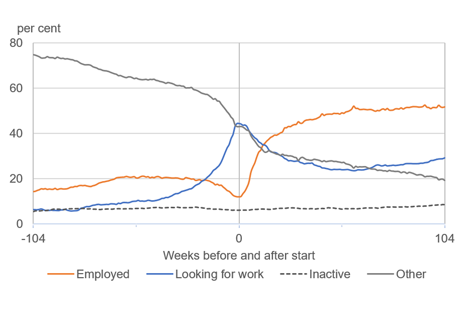
Note: The changes before and after starting the programme cannot be attributed to the programme. To understand the impact of the programme it must be compared to a counterfactual.
3.6 Comparison pool selection and Pseudo-start date assignment
In preparation for carrying out matching methods it is necessary to define a population of non-participants, known as a comparison pool, from which the final, matched comparison group will be selected. The initial selection criteria used to do this should mirror as closely as possible the selection and eligibility criteria for the participant group under consideration. For example, if the intervention being evaluated is only open to JSA claimants in the West Midlands who have been claiming for at least three months and are aged under 25, then that may be the starting point for the comparison pool. Care must be taken when choosing the region(s) from which to select a comparison pool. Local factors such as the availability of employment and public transport, levels of disadvantage, etc. all have an impact on the likelihood of someone finding and maintaining employment. For these reasons it is generally desirable to seek a comparison pool from the same region(s) as the programme in question.
However, if the programme’s reach or coverage was sufficiently large within a region, one may question why otherwise eligible individuals did not participate in the programme and whether they are suitable for the comparison pool. In such situations a comparison pool must be taken from outside the region, and attempts must be made to account for the local factors mentioned above.
In general, the programmes being evaluated will involve participants starting the programme at different times, perhaps spread over several years. Typically, the programme start date[footnote 11] is used as a reference point to base the measurement of outcomes. Once a comparison pool has been selected it is necessary to assign a date to each non-participant, known as a pseudo-start date, that can be used in place of the intervention start dates. The precise methods for doing this will vary from evaluation to evaluation depending on the nature of the intervention. Where an intervention has very specific start times and is focused on very specific groups[footnote 12] the decisions may be quite straight forward. Typically, this is not the case and careful consideration must be given to the selection of the comparison pool and the assignment of dates to ensure that bias is not introduced.
A general method for assigning the pseudo-start dates is to take the real start dates of the participant group and assign them randomly to the comparison pool in such a way that the distribution of the pseudo-start dates and real start dates match between the two groups. This ensures that any changes over time in the rates of recruitment for the participant group are reflected in the comparison pool.
Alternative methods for assigning the pseudo-start dates were explored during the development of the Data Lab and the sensitivity of impact estimates to the different methods were explored and found not to make much difference. This is discussed further in Appendix B.
Chapter 4 Analysis
4.1 Descriptive analysis
As mentioned previously, all evaluations undertaken by the Data Lab team include a descriptive analysis. This involves calculating a series of summary statistics, exploring the following topics:
-
the likely representativeness of the findings, given the percentage of participants who can be found in administrative data sources
-
the background characteristics of participants and location at the point when they start their participation in the intervention
-
employment and benefit history prior to starting on the intervention
-
participation in the intervention, including the distribution of start dates and any information supplied by User Organisations on the nature, duration, and intensity of participation
-
outcomes for participants, both for the primary outcome measure(s) and any secondary outcomes identified by User Organisations. The reasons for seeking to identify primary and secondary outcomes are explained in the following section
-
a comparison of information on participants supplied by User Organisations with information observed from Data Lab sources to assess consistency
The summary statistics would also highlight any variables which could not be observed for a high proportion of participants as this may limit the usefulness of such variables.
There may be instances where the period over which impacts on the primary outcomes are expected to emerge extends beyond the time-period that can be observed for all participants in the available data. In these cases, summary statistics on each of these topics are reported both for all participants and the subset for whom the primary outcomes can be observed in full. The statistical significance of any differences in characteristics between the two groups is calculated[footnote 13]. This analysis provides an insight into whether those who participated in the intervention at an earlier point in time have different characteristics to later participants. If this is the case, it suggests that the impact estimates for this early cohort may not be representative of the impact of the intervention on the wider pool of participants.
Where impact evaluation is likely to be possible some additional descriptive analysis is carried out for the comparison pool. This includes looking at the number of potential comparators who meet the eligibility criteria for the intervention. In general, having a large comparison pool will help in detecting any impact from the intervention. This is because a larger comparison pool will lead to lower standard errors and less uncertainty in the matched participant and comparison group estimates.
Finally, the descriptive analysis also assesses whether there are notable differences between participants and the comparison pool in terms of background characteristics, employment and benefit history and outcomes prior to matching. This includes identifying any differences between the two groups in the percentage of cases where information is missing and any key characteristics which cannot be observed for participants and/or the comparison pool.
4.2 Impact evaluation using propensity score matching
4.2.1 The methodology
Where it is possible to proceed to a full impact evaluation[footnote 14], this will be done using matching methods. As noted earlier, the reasons for focusing on this approach are set out in a literature review. The initial aim was to implement a method likely to be suited to producing a robust estimate of impact for a sizeable proportion of the interventions carried out by User Organisations. Over time, the range of methods used to estimate the causal impact of interventions may be expanded to cover a wider range of intervention types. Details of the approaches under future consideration are provided in the literature review. The priority will be to develop additional methods which are likely to apply to the largest number of evaluations. Other future plans include using additional administrative datasets from within DWP and other government departments, with the aim of evaluating the impact of interventions across a wider range of policy areas.
Propensity Score Matching (PSM) was chosen as the initial focus after a review of evaluations of active labour market programmes. This review suggested that with rich administrative data, PSM is most likely to be suited to evaluating the impact of a wide range of interventions where participation is voluntary. The credibility of the approach depends on being able to control for the range of factors likely to affect whether an individual participates in the programme, as well as the outcomes they are likely to attain. Provided all the factors that determine outcomes and participation in the intervention are accounted for in the analysis, any differences between the outcomes of participants and the matched comparison group can be attributed to the impact of the intervention. Where it is not possible to account for key factors that are likely to affect participation and outcomes, some of the differences in outcomes may be due to unobserved factors, rather than only the impact of participation in the intervention.
In practice it is not possible to explicitly account for all factors that might affect participation and outcomes as some may be unobserved in the available data. For example, a participant’s motivation to join a programme is often unobserved. Those who choose to participate in voluntary programmes may also have a higher level of motivation to find work than non-participants and thus be more likely to experience positive employment outcomes. Failing to take account of differences in motivation between participants and non-participants could lead to the estimate of impact being overstated. Also, factors that make it more difficult for individuals to work, such as having health problems or caring responsibilities, may also limit their ability to participate in an employment programme. If comparators are selected from non-participating individuals with more barriers to work than those who do participate, the impact of the intervention could be overstated.
In other cases, omitted characteristics may result in the impact of the intervention being underestimated. For example, those with a criminal record might have more need to participate in a voluntary programme in order to find employment but may also find it harder to get a job following participation. If it is not possible to observe whether participants and those in the comparison pool have a criminal record, this could lead to bias in the impact estimates.
The Data Lab aims to control for a sufficient number and range of relevant observed characteristics, so that it is reasonable to expect that after matching, the outcome is likely to be independent of the treatment (known as the Conditional Independence Assumption (CIA)). For example, taking into account an individual’s labour market history has been shown to be a valid proxy for unobserved but relevant characteristics such as personality traits and motivation (Caliendo, et al., 2014). The matching variables also include measures likely to capture potential barriers to work, such as having dependent children or being a lone parent.
It is also important to consider if the outcomes of the comparison group are affected either by the focal intervention or other interventions available at the same time. This can arise in the following circumstances:
-
when there is nothing to prevent the comparison pool from receiving the focal intervention in the period in which outcomes are observed
-
when the focal intervention affects outcomes for the comparison pool in either a positive or negative way. There may be positive spill-over if any benefits from the intervention improve outcomes for the comparison pool, for example, if participants were to share information and advice that they received as a result of participation with others in similar circumstances. Alternatively, displacement may occur if the intervention increased the likelihood of participants finding work, but employers were then less likely to employ those in the comparison pool. The estimate of counterfactual outcomes could bias the impact estimates in either of these cases
-
when other interventions available to participants and the comparison pool are designed to affect the same outcomes but where participation by either group is unequal – known as contamination. This may be the case if participating in the focal intervention is particularly time-consuming and reduces the ability of participants to engage in other activities. If the comparison pool makes more use of alternative programmes designed to affect similar outcomes, this may affect the robustness of the estimated counterfactual
The probability of satisfying the requirements underlying matching methods depends on the nature of the intervention and the eligibility criteria. However, the coverage of the linked administrative datasets available in the Data Lab, combined with access to a large potential comparison pool, means there is a good chance of meeting the assumptions underlying PSM for many of the interventions offered by potential User Organisations. The sections which follow describe each of the steps in the process of estimating the causal impact of interventions using PSM, as implemented by the Data Lab team.
4.2.2 Deciding on the approach to the analysis
Prior to conducting an impact analysis, the Data Lab team must assess the plausibility of constructing a comparison group that satisfies the conditional independence assumption that underlies PSM. As described above this assessment will be based on the nature of the programme and the outcome measures of interest, and how well these align to the data available as well as factors such as sample size and regional coverage of the programmes. Where it is decided that an impact evaluation is not appropriate the team will endeavour to provide descriptive analysis, detailing the characteristics, benefit and employment histories, and outcomes of programme participants without an assessment of the causal impact.
4.2.3 Identifying suitable outcome measures
When conducting an impact evaluation the larger the number of outcome measures, the greater the likelihood that some statistically significant impact estimates will be spurious (known as either false positives or false negatives). For this reason, the evaluation reports focus on one or two primary outcomes considered most likely to be affected if the intervention works as intended. These primary outcomes are identified before any impact estimates are produced.
Since the Data Lab is targeted at programmes supporting people into employment, most evaluations will likely include at least one employment related primary outcome measure. Two key examples of these are:
-
the number of weeks spent in employment in a specific time-period (typically one or two years) following individuals starting a programme. The impact in this case would be the difference in the mean number of weeks between the matched participant and comparison groups
-
the percentage of each group in employment at specific time points (for example six, 12 or 24 months) after starting a programme. The impact in this case would be the percentage point difference between the percentage of each group in employment at the chosen time point
Similar measures can be constructed for the other categories defined in section 3.5.2: Looking for work, Inactive or Other. One can also look deeper into the impacts of a programme by investigating the transitions between these categories at certain time points and the differences caused by the programme.
For evaluations that include DfE data it is possible to measure the percentage of each group in education and training at specific time points. These can be combined with employment information to create a flag indicating if an individual is “not in employment, education of training” (NEET), an important measure for some programmes.
4.2.4 Matching variables
In the development phase of the Data Lab, a list of potential matching variables suitable for many of the interventions delivered by User Organisations was compiled. Drawing on extensive experience within DWP of carrying out such analysis a standard set of matching variables was selected from this longer list. These were the indicators thought most likely to determine both the likelihood of participating in an intervention and shaping the outcomes experienced by participants and the comparison pool, across a wide variety of employment-related interventions. The standard set of matching variables covers the following characteristics:
-
individual characteristics: sex, age in years at the time of starting the intervention, age squared, and whether someone has a restricted ability to work (RATW)
-
family circumstances: whether lone parent, whether any dependent children, whether partnered
-
employment and benefit history: labour market status at the time of starting on the intervention. Including, in the two years prior to starting on the intervention:
- labour market status in each quarterly period
- whether in receipt of individual benefit types or employer
- whether sanctioned
- whether participated in the work programme
-
the timing of participation in the intervention: intervention start month and year
Appendix A provides a list of matching variables drawn from DWP, HMRC and DfE sources. Where the descriptive analysis shows that information is missing for more than 5 per cent of individuals on any of the matching variables, a dummy variable (coded to one for missing cases and zero otherwise) is derived and added to the list of matching variables.
In the first stage of the impact analysis, the Employment Data Lab team consider whether the standard set of matching variables based on DWP and HMRC data is likely to be adequate given the nature of the intervention. For example, if the comparison pool must be selected from out of area, the list of matching variables might be extended to include information on area-level factors that might impact outcomes. Evaluation outputs include details of any supplementary matching variables used.
4.2.5 Estimating propensity scores
Having identified the full range of variables likely to determine whether an individual participates in the intervention and likely to influence the expected outcomes from participation, the next step is to estimate propensity scores for all participants and those in the comparison pool. This involves using a regression model to estimate the likelihood that an individual with a given set of characteristics participates in the intervention.
The approach used in the Employment Data Lab is to estimate a probit model[footnote 15] based on the standard normal distribution, where the dependent variable takes a value of one for individuals known to have participated in the intervention and zero for individuals in the comparison pool. The characteristics described in the previous section (on matching variables) are used as independent variables in the probit regression. The statistical software package Stata is used for this purpose, and the “probit” command in particular.
Having fitted a probit regression to the data, the next step is to estimate a propensity score (the probability of participating in the intervention), for all individuals, based on their observed characteristics. For example, it may be the case that men aged between 18 and 24 are much more likely to participate in the intervention than women aged 50 or more. If this is the case, younger men will have a higher propensity score than older women, irrespective of whether a given individual in either group did in fact participate in the intervention. The propensity score is estimated by using the fitted regression model to predict the likelihood that each individual participates in the intervention and is therefore generated for all members of the participant and comparison groups.
4.2.6 Matching
After estimating propensity scores, the next step is to identify matched comparators for the programme participants. This is done by identifying comparators with a similar propensity score to the propensity score of a given participant. There are a variety of ways of carrying out the matching - referred to as different matching estimators.
A range of matching estimators are used in the analysis and the one deemed to give the closest match between the groups is chosen. This decision is based on the measures of balance (see the next section) and is made before any impact estimates are generated. The matching estimators used include kernel matching using Epanechnikov and normal kernel types, nearest neighbour matching and radius matching. A range of different bandwidths (between 0.001 and 0.06) and number of nearest neighbours (from 20 to 100) are explored. The literature review provides a detailed description of each of the different types of matching estimator. The data lab team use the “psmatch2” (Sianesi & Leuven, 2003) package within Stata to perform the matching.
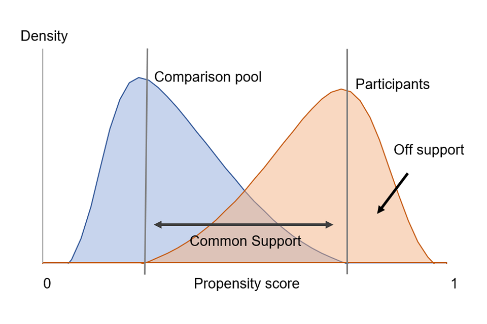
If the propensity scores for some of those who participated in the intervention are higher or lower than any individuals in the comparison pool, it is not possible to identify matched comparators for these participants. They are referred to as off support and are excluded from further analysis. The more participants that are off support the less representative are the impact estimates, so it is desirable that this is kept to a minimum.
Figure 4.1: Schematic showing overlapping distributions of propensity scores of a hypothetical participant and comparison group
The overlapping range is the region of common support. The participants that do not overlap with the comparators are off support.
4.2.7 Assessing balance
Having carried out the PSM, it is necessary to consider whether the participant and matched comparison groups appear similar in terms of their characteristics across the full range of matching variables. If there are sizeable differences in the characteristics of the two groups after matching, this suggests that the estimate(s) of impact(s) may be unreliable. If these differences cannot be addressed by adjusting the model parameters such as the matching estimator or bandwidth used, then it may not be appropriate to continue.
The Data Lab team compare the characteristics of participants ‘on support’ to those of the matched comparison group. The mean standardised bias (MSB) is calculated for each characteristic. This provides an indication of the extent to which the characteristics of the two groups differ after matching, taking into account variation within each of the groups[footnote 16].
As well as considering the magnitude of the MSB for each of the matching variables, the Data Lab team take into account whether the differences in characteristics which remain after matching are statistically significant. Both the statistical significance and magnitude of the MSB are considered when deciding whether the matched comparison group is likely to provide a robust estimate of counterfactual outcomes for participants, as even if the MSB is statistically significant, it may have little bearing on the impact estimates if the magnitude of the bias is small. Given the extensive list of matching variables used by the Data Lab team, the median and maximum standardised bias are calculated as an indicator of the scale of bias across the full range of matching variables
The Data Lab team also assess the extent to which the matching is successful in ensuring that the matched comparison group have similar characteristics to participants on support by computing Rubin’s B and R statistics. These are both overall indicators of the balance between the two groups across the full range of matching variables. They provide information on how different the propensity scores are between the matched participant and comparison groups. Rubin’s B[footnote 17] summarises the extent to which the mean values of the propensity scores are different and Rubin’s R[footnote 18] provides information on the variances. The rule of thumb suggested by Rubin is that B should be less than 25, and R should be between 0.5 and 2 (Rubin, 2001).
4.2.8 Estimating impact
Provided the participant and matched comparison groups appear similar in terms of observed characteristics, the Data Lab team use outcomes for the matched comparison group to estimate counterfactual outcomes for those who take part in the intervention. This estimate of the counterfactual is compared with actual outcomes for participants to estimate the impact of the intervention. This is achieved by simply subtracting the mean value for the matched comparison group from the mean value for the matched participant group.
As with the descriptive analysis, p-values and the statistical significance of the findings are considered, although these are approximate in the current approach to the analysis[footnote 19]. Having defined the matching estimator and produced the impact estimates, the analysis carried out using the different matching estimators and varying the closeness of the match required between participants and the comparison pool can also provide an indication of the robustness of the results.
As mentioned earlier, the analysis focuses on the impact of the intervention on one or two primary outcomes to reduce the likelihood of spurious findings, which are more likely to arise when estimating the impact of an intervention on many outcome measures. User Organisations are also asked when impacts are expected to emerge. This informs the period over which impact estimates are calculated.
4.3 Reporting
All Data Lab reports will be published as a condition of participation in the service. This reduces the risk of publication bias and recognises that there is often as much to learn from evaluations of less successful programmes as those of successful ones. All outputs follow a consistent format and can be found on the Employment Data Lab reports page.
The reports will focus on the primary outcome measures agreed with User Organisation prior to starting the analysis. Other additional and standard outcome measures will also be included in the report for completeness. Where it has not been possible or appropriate to generate an impact estimate, this will be clearly stated, and outcomes information will be provided instead.
Recognising that the Data Lab will be evaluating one facet of what can often be quite holistic programmes with a wide range of aims and objectives, User Organisations will have the opportunity within each report to describe their programme in their own words and respond to the analysis.
4.3.1 Statistical significance
Differences are labelled as statistically significant where the likelihood of observing that result by chance, when in fact there is no genuine underlying difference, is less than a set threshold. In the Data Lab reports, this threshold is set at 5 per cent. In addition to labelling statistically significant results, p-values are reported to show the probability of incorrectly rejecting the null hypothesis to provide a more detailed insight into the level of confidence in the findings.
4.3.2 Statistical disclosure control
To ensure that personal information is not disclosed all reports will undergo (risk based) statistical disclosure control prior to publication. Each table, plot or figure will be reviewed in relation to their disclosure risk and the context in which the data are presented. Where there is deemed to be a risk, action will be taken to suppress the data to reduce this risk. Typically, this will involve suppressing summary statistics that relate to very low (or high) numbers of individuals and carefully reviewing minima and maxima.
References
Ainsworth, P. & Marlow, S., 2011. Digital Education Resource Archive (DERA). [Online] Available at: https://dera.ioe.ac.uk/10322/1/ihr3.pdf
Caliendo, M., Mahlstedt, R. & Mitnik, O., 2014. Unobservable but unimportant? The influence of personality traits (and other usually unobserved variables) for the evaluation of labour market policies.. IZA.
Rubin, D., 2001. Using Propensity Scores to Help Design Observational Studies: Application to the Tobacco Litigation. Health Services and Outcomes Research Methodology 2, Volume (December) 169-88.
Sianesi, B. & Leuven, E., 2003. PSMATCH2: Stata module to perform full Mahalanobis and propensity score matching, common support graphing, and covariate imbalance testing. [Online] Available at: http://ideas.repec.org/c/boc/bocode/s432001.html
Ward, R., Woods, J. & Haigh, R., 2016. gov.uk. [Online] Available at: https://assets.publishing.service.gov.uk/government/uploads/system/uploads/attachment_data/file/508175/rr918-sector-based-work-academies.pdf
Appendix A Variables
Table A.1 Variables available for use in the Data Lab analysis
Some variable names listed below include square brackets with characters inside. This is shorthand notation indicating that there are multiple different variables denoted by the different options in the square brackets - e.g. [w, l, i, o]_start indicates that the are four similar variables called: w_start, l_start, i_start and o_start.
Scroll right to see full table.
| Name | Type | Options | Description |
|---|---|---|---|
| encnino, ccnino | Character | Unique identifier (encrypted NINO). | |
| pilot | Numeric | 1,0 | Participant (1) or comparator (0). |
| treated | Numeric | 1,0 | Participant (1) or comparator (0). |
| intervention_start_date | Date | Date participant started the intervention. This is the pseudo-start date for the comparison group. | |
| intervention_year | Numeric | integer | Year in which they started the intervention, e.g. 2017. |
| intervention_month | Numeric | integer | Month of the year in which they started the intervention, e.g. July would be 7. |
| f_dob | Date | Date of birth. | |
| f_sex | Numeric | 1,0 | Male (1) or female (0). |
| f_age | Numeric | Integer | Age at intervention start date, in years. |
| f_age_sq | Numeric | integer | Age at intervention start date, in years, squared. |
| f_ratw_start | Numeric | 1,0 | Flagged as having a restricted ability to work (1) or not (incl. unknown) (0) at programme start. Only available for people on specific benefits. |
| f_ratw | Numeric | 1,0 | Flagged as having a restricted ability to work (1) or not, or missing (0) during the most recent benefits spell (without a missing value) in the two years before start. Only available for people on specific benefits. |
| f_loneparent | Numeric | 1,0 | Flagged as being a lone parent (1) or not, or missing (0) during the most recent benefits spell (without a missing value) in the two years before start. Only available for people on specific benefits. |
| f_partner | Numeric | 1,0 | In a relationship (1) or not, or missing (0) during the most recent benefits spell (without a missing value) in the two years before start. Only available for people on specific benefits. |
| f_children | Numeric | 1,0 | Has dependent children (1) or not, or missing (0) during the most recent benefits spell (without a missing value) in the two years before start. Only available for people on specific benefits. |
| f_dwp_ethnicity_[asian, black, chinese, mixed, other, white, british, not_given, missing] | Numeric | 1,0 | Flags indicating ethnicity as recorded in various DWP datasets. These flags are not necessarily mutually exclusive. |
| f_miss_[ratw, loneparent, partner, children] | Numeric | 1,0 | Flag indicating that the specified variable (described above) is missing |
| lauanm | Character | Geographic location variable: Local Authority name. At intervention start. | |
| nuts[1,2,3]nm | Character | Geographic location variable: Nomenclature of Units for Territorial Statistics 2013 Level [1,2,3] (NUTS[1,2,3]). At intervention start. | |
| coa_2001_t | Character | Geographic location variable: Census output area 2001. At intervention start. | |
| coa_2011_t | Character | Geographic location variable: Census output area 2011. At intervention start. | |
| ctynm | Character | Geographic location variable: County Name. At intervention start. | |
| [ear, uer, p_po, p_eo, p_st, p_nvq[1,2,3,4]p]_year | Numeric | Various | Rates of the following variables, in the geographic location (NUTS3NM) of the person at start, during the intervention year. Derived from NOMIS data. ear - economic activity rate; uer - employment rate; p_po - percentage in professional occupations; p_eo - percentage in elementary occupations; p_st - percentage in skilled trades; p_nvq[1,2,3,4]p - percentage with at least NVQ level [1,2,3,4] qualification |
| [ear, uer, p_po, p_eo, p_st, p_nvq[1,2,3,4]p]year_m[1,2] | Numeric | Various | as above, but for the [1,2] year(s) before the intervention year |
| missing_[[ear, uer, p_po, p_eo, p_st, p_nvq[1,2,3,4]p]year_m[1,2]], | Numeric | 1,0 | Flag indicating that the specified variable (described above) is missing |
| cluster | Numeric | 1-14 | Number indicates location in one of 14 clusters of local authorities (GB only). A range of local labour market characteristics were used in the cluster analysis. |
| cluster[1-14] | Numeric | 1,0 | Flag indicating which local labour market cluster an individual was located in at programme start. |
| [w, l, i, o]_start | Numeric | 1,0 | Flag indicating labour market status (w - employed, l - looking for work, i - inactive, o - other) at start. These categories are not mutually exclusive. |
| [w, l, i, o]_week_m1 | Numeric | 1,0 | As above, but for 1 week prior to start |
| [w, l, i, o]month[m,p]_[3,6,9,12,15,18,21,24] | Numeric | 1,0 | As above but for quarterly time points (last day of the quarter) before [m] and after [p] start, spanning two years either side of the start. |
| [w, l, i, o]monthly[m,p]_[1-24] | Numeric | 1,0 | As above but for monthly time points (last day of the month) before [m] and after [p] start. |
| [w_x, l_x, i_x, o_x, l_w, i_w.l_i]_start | Numeric | 1,0 | Flag indicating mutually exclusive labour market status combinations (w - employed, l - looking for work, i - inactive, o - other) at start. For example w_x means employed only, l_w means in the looking for work and employed categories. |
| [w_x, l_x, i_x, o_x, l_w, i_w, l_i ]_week_m1 | Numeric | 1,0 | As above, but for 1 week prior to start |
| [w_x, l_x, i_x, o_x, l_w, i_w.l_i]month[m,p]_[3,6,9,12,15,18,21,24] | Numeric | 1,0 | As above but for quarterly time points (last day of the quarter) before [m] and after [p] start, spanning two years either side of the start. |
| [w_x, l_x, i_x, o_x, l_w, ]monthly[m,p]_[1-24] | Numeric | 1,0 | As above but for monthly time points (last day of the month) before [m] and after [p] start. |
| trans_01[2]_iw[ix, li, lw, lx, ox, wx]_iw[ix, li, lw, lx, ox, wx] | Numeric | 1,0 | Flag indicating a transition between the specified labour market categories between the start and 1 [1] or 2 [2] years later. e.g. a flag for trans_02_lw_wx, would indicate a transition between being in the looking for work and employed categories at start and moving to employed only 2 years later. |
| dur_[m,p]_[w,l,i,o]_q1[2,3,4,5,6,7,8] | Numeric | integer | Number of weeks with at least one day spent in the specified labour market category during each quarter [1-8] spanning the two years before [m] and after [p] programme start. |
| dur_[w,l,i,o]_[1,2]year | Numeric | integer | Number of weeks with at least one day spent in the specified labour market category during the first 1 [1] or 2 [2] years after programme start. |
| dur_[l_x, l_i, l_w, i_x, i_w, w_x]_[1,2]year | Numeric | integer | Number of weeks with at least one day spent in the specified labour market category during the first 1 [1] or 2 [2] years after programme start. |
| pat[to 8]_[jsa, esa, wb, dla, sda, pib, bb, is, ica, ib, bsp, uc_ee, uc_iws, uc_ltiw, uc_ltoow, uc_miss, uc_noreq, uc_wfi, uc_wprep, emp, sa, dlapip, hb, cb, ctc, wtc] | Numeric | 1,0 | 8 flags indicating a given sequence of the specified benefit or tax credit status during the 18 months prior to intervention start. |
| binary_[jsa, esa, wb, dla, sda, pib, bb, is, ica, ib, bsp, uc_ee, uc_iws, uc_ltiw, uc_ltoow, uc_miss, uc_noreq, uc_wfi, uc_wprep, emp, sa, dlapip, hb, cb, ctc, wtc][hist, fut] | Numeric | 1,0 | Flag indicating receipt of each benefit or tax credit at any time in the two years before [hist] or after [fut] intervention start |
| wks2emp_monthly_p_[6,12,24] | Numeric | integer | Number of weeks from programme start to start date of first employment (of greater than 5 days), calculated at [6, 12, 24] months. |
| dlapip_start | Numeric | 1,0 | Flag indicating being in receipt of DLA or PIP at intervention start |
| snc_[hist, imp]_flg | Numeric | 1,0 | Flag indicating if there is a recorded sanction in the two years prior to [hist] of after [imp] intervention start |
| wp_[start, hist, fut] | Numeric | 1,0 | Flag indicating participation in the Work Programme at programme start [start] or any time in the two years prior to [hist], or after [fut] programme start |
| ESF_[start, hist, fut] | Numeric | 1,0 | Flag indicating participation in an ESF programme at start [start] or any time in the two years prior to [hist], or after [fut] programme start |
| int_[start, hist, fut] | Numeric | 1,0 Flag indicating participation in a DWP employment programme at programme start [start] or any time in the two years prior to [hist], or after [fut] programme start | |
| PRAP_REF_[start, hist, fut] | Numeric | 1,0 | Flag indicating referral to, but not participation in, a DWP programme at start [start] or any time in the two years prior to [hist], or after [fut] programme start |
| [educ, c, a, h, neet]_start | Numeric | 1,0 | Flag indicating education status (educ-any, c - school, a - further education, and h- higher education) at start |
| [educ, c, a, h, neet]_week_m1 | Numeric | 1,0 | as above but 1 week prior to start |
| [educ, c, a, h, neet]month[m,p]_3[6,9,12,15,18,21,24] | Numeric | 1,0 | as above but at quarterly time points (on the last day of the quarter) before [m] and after [p] start spanning two years either side of the start. These categories are not mutually exclusive. |
| EthnicGroupMajor | Character | Various | Ethnicity group as recorded in school census (DfE) |
| EthnicGroupMinor | Character | Various | Ethnicity group as recorded in school census (DfE) - more detailed categorisation |
| f_dfe_ethnicity_[asian, black, chinese, mixed, other, white] | Numeric | 1,0 | Flags indicating ethnicity, derived from the above DfE ethnicity category variables. |
| trans_0[1,2][a,c,h,n,e][a,c,h,n,e] | Numeric | 1,0 | Flag indicating a transition between two education statuses (c - school, a - further education, h- higher education, e-education (any), w - employment and n - neet ) between the start and 1 [1] or 2 [2] years later. These categories are not mutually exclusive. |
| trans_01[2][xx, xw, xe, we][xx, xw, xe, we] | Numeric | 1,0 | Flag indicating a transition between being neet [xx], work only [xw], education only [xe] and in work and education [we] between the start and 1 [1] or 2 [2] years later. These categories are mutually exclusive. |
| sen_new | Numeric | 1,0 | Flag indicating the presences of an historic special educational needs designation |
| sen_PIT | Numeric | 1,0 | Flag indicating whether someone has had a special educational needs provision at any point between age 14 and 18 |
| fsm_new | numeric | 1,0 | Flag indicating the presences of an historic free school meal eligibility |
| fsm_PIT | Numeric | 1,0 | Flag indicating whether someone was eligible for free school meals at any point between age 14 and 18 |
| cla_flag | Numeric | 1,0 | Flag indicating being a care leaver or having been adopted. From the Key Stage 4, school census, and children looked after datasets of the NPD |
| cla_adopt | Numeric | 1,0 | Flag indicating being a care leaver or having been adopted. From the Key Stage 4 datasets of the NPD. |
| cin_flag | Numeric | 1,0 | Flag indicating having been a child in need. |
| uasc_flag | Numeric | 1,0 | Flag indicating whether someone has ever been an unaccompanied asylum seeking child |
| max_qual_start | Character | L0 - L8 | Variable recording the maximum qualification level achieved at programme start |
| level_[0,1,2,3,4,5,6,7,8]_start | Numeric | 1,0 | Flag indicating having achieved specified qualification at start. Lower qualification levels are back filled, for example someone with a level 4 qualification would have levels, 0,1,2,3 and 4 all flagged. |
| level_M1_start | Numeric | 1,0 | Flag indicating qualification level achieved is missing. |
| level_[0,1,2,3,4,5,6,7,8]_[1 year, 2 year, fut] | Numeric | 1,0 | Flag indicating having passed a qualification at specified level at any point during the specified time period after start. |
| exclusion | Numeric | 1,0 | Flag indicating presence on DfE exclusions datasets |
| exclusion_PIT | Numeric | 1,0 | Flag indicating presence on DfE exclusions datasets at any point between age 14 and 18 |
| permanent | Numeric | 1,0 | Flag indicating a permanent exclusion recorded in DfE exclusions dataset. |
| permanent_PIT | Numeric | 1,0 | Flag indicating a permanent exclusion recorded in DfE exclusions datasets at any point between age 14 and 18 |
| missing_[ethinicgroup, ethinicgroupminor, dfe_ethnicity[…], fsm_cla, cla_adopt, fsm_new, sen, sen_new, exclusion, permanent, ks4lan1st, level[…]_start, ] | Numeric | 1,0 | Flag indicating that the specified variable (described above) is missing |
| missing_[ fsm_pit, cla_flag, fsm_pit, sen_pit, exclusion_pit, permanent_pit, level[…][start,1year,2year,fut],qualification [1year,2year,fut],usac_flag] |
Numeric | 1,0 | Flag indicating that the specified variable (described above) is missing |
| CHAR_DOB | Date | Date of birth. | |
| CHAR_SEX | Numeric | 1,0 | Male (1) or female (0). |
| CHAR_AGE | Numeric | integer | Age at intervention start date, in years. |
| CHAR_AGE_sq | Numeric | integer | Age at intervention start date, in years, squared. |
| CHAR_INT_YEAR_[YYYY] | Numeric | 1,0 | Flag indicating if someone started the intervention in a given year, e.g. CHAR_INT_YEAR_2017 is equal to one if someone started in 2017. |
| CHAR_INT_MONTH_[1-12] | Numeric | 1,0 | Flag indicating whether someone started the intervention in a calendar given month [1-12]. |
| CHAR_CHILDREN | Numeric | 1,0 | Has dependent children (1) or not, or missing (0). Only available for people on specific benefits. |
| GEOG_CLUSTER_[1-14] | Numeric | 1,0 | Flag indicating which local labour market cluster an individual was located in at programme start. |
| SPELL_NEW_OTHER [m,p] [1-24] | Numeric | 1,0 | Flag indicating not enrolled in education, in employment, or in receipt of looking for work or inactive benefits during the month before [m] and after [p] start, spanning two years either side of the start. |
| SPELL_[WORK, LFW, Inactive, OTHER]_[m,p][1-24] | Numeric | 1,0 | Flag indicating labour market status (WORK - employed, LFW - looking for work, Inactive, OTHER) during the month before [m] and after [p] start, spanning two years either side of the start. These categories are not mutually exclusive. |
| SPELL_DUR_[M,P][1,2]YR_[WORK, LFW, Inactive, OTHER] | Numeric | integer | Number of months spent in the specified labour market category during the first 1 [1] or 2 [2] years before [M] or after [P] programme start. |
| SPELL_[jsa, esa, wb, dla, sda, pib, bb, is, ica, ib, bsp, uc_ee, uc_iws, uc_ltiw, uc_ltoow, uc_miss, uc_noreq, uc_wfi, uc_wprep, emp, sa, dlapip, hb, cb, ctc, wtc][hist, fut] | Numeric | 1,0 | Flag indicating receipt of each benefit or tax credit at any time in the two years before [hist] or after [fut] intervention start |
| SPELL_TIME_TO_WOR_[6, 12, 18, 24] | Numeric | integer | Number of months from programme start to start date of first employment (of greater than 5 days), calculated at [6, 12, 18, 24] months. |
| SPELL_TR_[01,02]Y_[W,L,I,O]_[W,L,I,O] | Numeric | 1,0 | Flag indicating a transition between the specified labour market categories between the start and 1 [01] or 2 [02] years later. e.g. a flag for SPELL_TR_02Y_L_W, would indicate a transition between being in the looking for work category at start and moving to the employed category 2 years later |
| PIT_SANC_[hist, fut] | Numeric | 1,0 | Flag indicating if there is a recorded sanction in the two years prior to [hist] of after [fut] intervention start |
| PIT_INT_[start, hist, fut] | Numeric | 1,0 | Flag indicating participation in a DWP employment programme at programme start [start] or any time in the two years prior to [hist], or after [fut] programme start |
| DFE_[educ, c, a, h, neet]_start | Numeric | 1,0 | Flag indicating education status (educ-any, c - school, a - further education, and h- higher education) at start |
| DFE_[educ, c, a, h, neet]_week_m1 | Numeric | 1,0 | as above but 1 week prior to start |
| DFE_[educ, c, a, h, neet]_month_[m,p]_[1-24] | Numeric | 1,0 | as above but at monthly time points before [m] and after [p] start spanning two years either side of the start. These categories are not mutually exclusive. |
| DFE_ethnicity_[asian, black, chinese, mixed, other, white] | Numeric | 1,0 | Flags indicating ethnicity, derived from the above DfE ethnicity category variables. |
| DFE_SEN | Numeric | 1,0 | Flag indicating the presences of an historic special educational needs designation |
| DFE_FSM | Numeric | 1,0 | Flag indicating the presences of an historic free school meal eligibility |
| DFE_CLA | Numeric | 1,0 | Flag indicating being a care leaver or having been adopted. From the Key Stage 4, school census, and children looked after datasets of the NPD. |
| DFE_CIN | Numeric | 1,0 | Flag indicating having been a child in need. |
| DFE_UASC | Numeric | 1,0 | Flag indicating whether someone has ever been an unaccompanied asylum seeking child |
| Dfe_level_[0,1,2,3,4,5,6,7,8]_start | Numeric | 1,0 | Flag indicating having achieved specified qualification at start. Lower qualification levels are back filled, for example someone with a level 4 qualification would have levels, 0,1,2,3 and 4 all flagged. |
| Dfe_level_[0,1,2,3,4,5,6,7,8]_[1year, 2year, fut] | Numeric | 1,0 | Flag indicating having passed a qualification at specified level at any point during the specified time period after start |
| DFE_exclusion | Numeric | 1,0 | Flag indicating presence on DfE exclusions datasets |
| DFE_permanent | Numeric | 1,0 | Flag indicating a permanent exclusion recorded in DfE exclusions datasets. |
| DFE_MISSING | Numeric | 1,0 | Flag indicating whether or not an induvial has a presence in the Longitudinal Educational Outcomes (LEO) dataset. |
| ANN_EARNINGS_YR[m,p][1,2,…] | Numeric | Integer | Annual earnings (£) in the specified tax year [1,2,…] before [m] or after [p] the tax year of programme start. |
| ks4_idaci | Numeric | Proportion | The Income Deprivation Affecting Children Index (IDACI) score measures the proportion of all children aged 0 to 15 living in income deprived families in a lower-layer super output area (LSOA). |
| GCSE_AA | Numeric | Integer | Number of A or A-star (or numeric equivalent) grades achieved at GCSE. |
| GCSE_B | Numeric | Integer | Number of B (or numeric equivalent) grades achieved at GCSE. |
| GCSE_C | Numeric | Integer | Number of C (or numeric equivalent) grades achieved at GCSE. |
| GCSE_D | Numeric | Integer | Number of D (or numeric equivalent) grades achieved at GCSE. |
| GCSE_E | Numeric | Integer | Number of E (or numeric equivalent) grades achieved at GCSE. |
| GCSE_FG | Numeric | Integer | Number of F or G (or numeric equivalent) grades achieved at GCSE. |
| ALEVEL_SUM | Numeric | Integer | Number of subjects studied at A-level. |
| ALEVEL_[MATH,CHEMISTRY,BIOLOGY,PHYSICS,HIST,ECON,PSYCH,MATH_FURT,ENG_LIT,GEOG,SOC,GOV_POLITICS,RE] | Numeric | 1,0 | Flag indicating A-level subjects [mathematics, chemistry, biology, physics, history, economics, psychology, further mathematics, English literature, geography, sociology, government and politics, religious studies] studied. |
| academic_framework | Numeric | Integer | Number of A-level subjects studied in either the Facilitating [modern foreign languages, ancient foreign languages, biology, chemistry, English literature, mathematics, further mathematics, pure mathematics, geography, history, human biology, physics] or Useful [ancient history, archaeology, classical civilisation, classics, computing, Welsh first language, economics, economics and business, English language and literature, environmental science, geology, government and politics, history of art, music, philosophy, psychology, religious studies, sociology, statistics] subjects groups[footnote 20]. |
| SPELL_[C,A,H]_[HIST_FUT] | Numeric | 1,0 | Flag indicating enrolment in education type at any time in the years (generally two) before [hist] or after [fut] intervention start. |
| russell_group_enrolled | Numeric | 1,0 | Flag indicating enrolment at a Russell Group university during the years after starting the programme. |
| russell_group_degree | Numeric | 1,0 | Flag indicating a degree was obtained from a Russell Group university during the years after starting the programme. |
| first | Numeric | 1,0 | Flag indicating a first class degree was obtained during the years after starting the programme. |
| upper_second | Numeric | 1,0 | Flag indicating an upper second class degree was obtained during the years after starting the programme. |
| lower_second | Numeric | 1,0 | Flag indicating a lower second class degree was obtained during the years after starting the programme. |
| third | Numeric | 1,0 | Flag indicating a third class degree was obtained during the years after starting the programme. |
Appendix B Note on pseudo-start date allocation
The baseline method for assigning pseudo-start dates in the Data Lab is to randomly assign the real start dates to the comparison pool in such a way that the distribution matches the participant group. A more complex method of assigning the pseudo-start dates was also explored. This follows the method employed by Ainsworth and Marlow (Ainsworth & Marlow, 2011) and Ward, et al (Ward, et al., 2016) and attempts to link the assignment of a pseudo-start date to the date an individual started a labour market spell of relevance (for example a JSA spell). This method goes some way to aligning the labour market histories prior to matching and might be particularly relevant for programmes that require people to be on a specific benefit to be eligible to participate.
In this method the participant and comparison groups are first categorised into cohorts depending on when they started a spell of interest. This might be the calendar month, or quarter in which they started a specific JSA spell, for example. It is then within these cohorts that the pseudo-start dates are allocated in a way that matches the distribution of participant start dates within each respective cohort[footnote 21].
As part of the development of the Data Lab and following Ainsworth and Marlow (Ainsworth & Marlow, 2011), the sensitivity of Data Lab results to the method of pseudo-start date was explored. The two approaches were compared, and like Ainsworth and Marlow the method of pseudo-start date allocation made little difference. As a result, the simpler approach was adopted as the baseline method in the Data Lab.
-
In technical terms, a primary objective of the Data Lab is to produce studies with high internal validity. It is outside the scope of the Data Lab to consider the external validity of research findings i.e. whether the same impacts could be expected in different circumstances, such as at a different time or in a different area. ↩
-
It is assumed that participants would have had access to the usual range of support available to those with similar characteristics, known as business-as-usual. ↩
-
Details on how the participant data is linked to the administrative data is discussed in section 3.5.1. ↩
-
This is not full anonymisation as it would still be possible to re-identify participants if required. ↩
-
Via the Longitudinal Education Outcomes (LEO) data match. See ‘Longitudinal education outcomes study: how we use and share data’ for further information. ↩
-
In this chapter “linking” and “matching” mean the same thing. Not to be confused with propensity score matching discussed later in this document. ↩
-
Some data sets, such as the DfE datasets which has already been linked to DWP data and hence has NINOs, will only be used as and when their use is justified and consistent with the legal gateways under which the datasets were shared with DWP. ↩
-
People on UC fall into one of six conditionality regimes depending on their personal circumstances. Which of these groups they are placed into will determine what activities they are required to do (if any) as part of their claim. ↩
-
People on UC Working – no requirements may also fall into this category if they do not have an associated employment record. The reason for this is that someone may be placed in this category based on the financial situation of a co-claimant. ↩
-
Several other benefits also fall into this category, though the numbers of people on these benefits is small, these include: Income Support, Incapacity Benefit, Severe Disablement Allowance and Passported Incapacity Benefit. ↩
-
Or in some cases other reference points may be used such as a programme end date or perhaps a release date if the programme takes place during a prison spell. ↩
-
For example, a programme involving 18-year olds who all start the programme on 1 September each year. ↩
-
See section 4.3.1 for further information on the use of statistical significance in the Data Lab. ↩
-
The assessment of if an impact evaluation is possible is discussed in section 4.2.2. ↩
-
A probit model a type of statistical model used to estimate the probability of an event occurring given a set of factors that may influence the event happening, for example, the probability of participating a programme, given a set of personal characteristics. ↩
-
The difference in means between the treatment and matched comparison groups is divided by the square root of the mean sample variance to calculate the mean standardised bias. It is expressed as a percentage. ↩
-
Rubin’s B is the absolute standardized difference in the means of the linear index of the propensity scores for the participant and comparison groups. ↩
-
Rubin’s R is the ratio of participant to comparison group variances in the propensity scores. ↩
-
The Data Lab team currently use the approximate standard errors generated by the psmatch2 command in Stata for the calculation of statistical significance and confidence intervals, The preferred method of calculating standard errors for kernel matching uses bootstrapping. This is a process intensive technique when combined with PSM and is prohibitive for larger sample sizes. During the development of the Data Lab the approximate methods of calculated standard errors were compared to those generated from bootstrapping and found to be similar. ↩
-
Subject groupings come from the 2016 Russell Group publication Informed choices: A Russell Group guide to making decisions about post-16 education. ↩
-
When using this method, care must be taken when selecting the spell of interest for the comparison group so that bias is not introduced. Care must also be taken to ensure that the distribution of each group among the cohorts is similar. ↩