Literature review and methodological background to the Employment Data Lab

Question 1

Executive Summary

Accepted Answer

The purpose of the DWP Employment Data Lab

The DWP Employment Data Lab has been set up to evaluate the impact of employment-related interventions delivered by external organisations. The Employment Data Lab will use linked administrative data to produce robust evidence on the causal impact of these programmes to contribute to the evidence on the effectiveness of different types of employment intervention. Participation in the programmes is on a voluntary basis.

External organisations will be asked to supply information on the individuals they work with to the Employment Data Lab team. This will be used to obtain individual-level records for programme participants from DWP and HM Revenue and Customs (HMRC) sources. At a minimum, the Employment Data Lab will seek to use this information to produce a descriptive analysis of the characteristics and outcomes of programme participants. Wherever possible though, the aim will be to estimate the causal impact of the intervention.

In the short term the Employment Data Lab wishes to develop a streamlined methodological approach which is suited to producing robust and defensible causal impact estimates for a wide range of different programmes relatively quickly. This report seeks to identify a suitable approach, based on a review of past evaluations of active labour market programmes, as well as the work of the Justice Data Lab, which has similar aims to the Employment Data Lab. It also suggests ways in which the Employment Data Lab could expand and strengthen its work in the future.

The data

In its initial phase of development, the Employment Data Lab will have access to the information from the following datasets:

DWP administrative datasets, which provide details of spells on DWP benefits and employment programmes as well as characteristics of DWP customers
HMRC Tax System, which provides details of employment spells
Department for Education administrative datasets, which provide details on time spent in education and training, qualifications obtained and other associated characteristics, such as eligibility for free school meals, or special educational needs status

The intention is to link to more datasets held by other government departments in the future.

Lessons learned from past evaluations of active labour market programmes

The review of past evaluations of active labour market programmes highlights the need to obtain standardised information from the organisations delivering the intervention before commencing the analysis. This will assist in deciding whether it will be possible to produce causal impact estimates, and where this is possible, refining the design of the impact evaluation.

Propensity Score Matching (PSM) has been widely used in past evaluations of active labour market programmes where participation is voluntary and is the method most likely to be suited to the work of the Employment Data Lab. This report highlights the key statistics and sensitivity checks that should be reported to demonstrate that the matching process has been effective and whether the estimate of impact is likely to be robust. It also highlights a number of other methods which have been used in past evaluations of active labour market programmes which may be of relevance to the work of the Employment Data lab, depending on the nature and scale of the intervention being evaluated.

Whilst PSM is most likely to be appropriate to the work of the Employment Data Lab in the initial phase of development, any future expansion in the work of the Employment Data Lab should consider the feasibility of implementing these alternative methodologies to make it possible to evaluate the impact of a wider range of interventions.

Lessons learned from the Justice Data Lab

The Justice Data Lab provides a model of how administrative data can be used to carry out impact evaluations of interventions implemented by third parties. It provides a working, peer-reviewed example of the information required from delivery organisations and ways of presenting outputs. This includes identifying a set of outcome measures and matching variables which are likely to reflect the aims of delivery organisations, the use of standardised templates for collecting information on the intervention, deciding on minimum thresholds for reporting and the use of visual outputs, with clear caveats.

The Employment Data Lab could further strengthen the approach taken in the Justice Data Lab by considering alternative ways of identifying the most appropriate choice of matching variables and doing more to demonstrate that the treatment and comparison groups are well-matched.

A proposed methodology for the Employment Data Lab

It would be beneficial for the Employment Data Lab to draw up a comprehensive list of outcome measures that could be observed in the DWP and HMRC administrative data, drawing on the review of evaluations of active labour market policies provided in this report. Prior to obtaining data on programme participants from delivery organisations it would be helpful to develop a template which collects basic information on the nature of the intervention, its aims and those targeted by the intervention, in a standardised format. This should include:

A brief description of the intervention
Details of any eligibility criteria that individuals have to meet before they are able to receive the intervention
Any other restrictions on eligibility, such as whether the programme is only available in particular areas
The numbers of individuals who have received support. Ideally this would be a detailed breakdown by month
The number of treated individuals where a national insurance number is recorded
Identifying one or two primary outcomes expected to be affected by the intervention, from the list supplied by the Employment Data Lab
Specifying any secondary outcomes likely to be affected (again drawing from the Employment Data Lab list)
The timeframe over which any short- medium and longer-term impacts are expected to be seen if the programme is effective

The template used by the Justice Data Lab provides an example of the sort of information required and how it could be collected. This information can be used to assess the likelihood of being able to estimate the impact of the intervention, or whether it may be necessary to wait for any impacts to emerge.

The preliminary phase of work should also include drawing up a list of potential matching variables, again drawing on the review of past evaluations of active labour market programmes which have used DWP and HMRC data provided by this report. This could usefully distinguish between matching variables which are likely to be essential in any evaluation of an employment programme and those which would be suited to particular types of intervention, for example those with a focus on retraining for older workers.

In the first instance, it is recommended that the Employment Data Lab focuses on evaluating the impact of programmes which are suited to the use of PSM. It will be necessary to develop a standardised way of carrying out the analysis and presenting the results. This should include measures to demonstrate the match between the treatment and comparison groups (such as computing the mean standardised bias on the matching variables) and reporting Rubin’s B and R. The output should also show the proportion of the treatment group for whom close matches are found (the percentage on support). As standard, it would also be advisable to carry out some basic checks on the sensitivity of the impact estimates to varying the choice of matching estimator and the required closeness of the match. It would also be beneficial to calculate Rosenbaum Bounds.

Once the model of conducting PSM is established, the Employment Data Lab could be developed in a number of ways:

Refining the approach to the selection of matching variables and balancing the characteristics of the treatment and comparison groups
Exploring the sensitivity of the findings to using alternative methods to estimate impact, such as machine learning
Considering the value of using CEM to evaluate the impact of larger-scale interventions
Increasing the range of evaluation techniques to be used by the Employment Data Lab to capture the impact of a wider range of interventions

A further longer-term option would be exploring the feasibility of making linked individual-level data available to third parties to carry out independent impact evaluations. This may be particularly useful in enhancing the range of interventions that can be evaluated, increasing capacity, and building a community of expert users who can contribute to quality assurance and the peer review of outputs.

Question 2

1 Introduction

Accepted Answer

1.1 About the DWP Employment Data Lab

1.1.1 Aims

The DWP Employment Data Lab has been set up to evaluate the impact of employment-related interventions conducted by external organisations, such as local authorities, charities, and private sector bodies. Participation in these interventions is on a voluntary basis. The aim is to produce robust evidence on the impact of a wide range of different types of intervention. By improving the evidence base the Employment Data Lab seeks to improve the effectiveness of employment programmes run both by DWP and by third parties. A further objective of the Employment Data Lab is to use existing data to enhance the public good.

1.1.2 The process

Subject to meeting General Data Protection Regulation (GDPR) requirements, external organisations engaged in delivering employment-related programmes will be asked to provide information on the individuals that they have worked with to the Employment Data Lab team. The team will use this information to identify individual-level records in Government administrative datasets for programme participants. Wherever possible, the Employment Data Lab team will seek to carry out an impact evaluation using quasi-experimental methods to estimate the causal impact of the intervention. The feasibility of using such methods is likely to depend on whether it is possible to identify a suitable comparison group or estimate the counterfactual (what would have happened to participants if they had not received support from the intervention) in some other way.

If it is not possible to form a credible estimate of the counterfactual a descriptive analysis of the characteristics and outcomes of programme participants will be reported. This will provide insights into the types of individuals who take up the intervention, their personal circumstances, their use of benefits, and their employment outcomes following participation in the intervention.

1.1.3 The Data

In its initial phase of development, the Employment Data Lab will have access to information from the following datasets:

DWP administrative datasets, which provide details of spells on DWP benefits and employment programmes as well as characteristics of DWP customers
HM Revenue and Customs (HMRC) Tax System, which provides details of employment spells
Department for Education administrative datasets, which provides details on time spent in education and training, qualifications obtained and other associated characteristics, such as eligibility for free school meals, or special educational needs status

It is hoped that it will be possible to expand the range of datasets which can be linked to DWP data in the future. This could potentially include information from the Ministry of Justice.

It takes time for each of the administrative datasets to be compiled and updated, so in most cases there is a delay of some months between an individual experiencing a particular outcome, and it being possible to observe this in each of the data sources. The delay is much greater in the case of the self-employment data, as individuals are not required to submit their self-assessment form until 9 months after the end of a given tax year.

1.1.4 Objectives

The immediate objective of the Employment Data Lab is to identify and implement a methodological approach which is suited to producing robust and defensible estimates of the causal impact of a range of different employment-related interventions. The aim is to develop a streamlined approach which can be used to produce evidence on the causal impact of interventions relatively quickly. This means devising computational syntax and outputs which can be easily adapted for each evaluation, whilst also ensuring that the methods are appropriate given the nature of the interventions.

Over the longer-term the aim is to expand the work of the Employment Data Lab to carry out evaluations of a wider range of interventions. This could involve expanding the number of techniques used and incorporating emerging methodologies. As the work of the Employment Data Lab becomes more established it may be possible to invest further in software, hardware, and training to support the use of a wider range of techniques.

1.2 Report objectives

This report seeks to inform the development of the Employment Data Lab in a number of ways:

Providing an overview of established methods of identifying the causal impact of policy interventions likely to be relevant to the work of the Employment Data Lab
Reviewing the use of quasi-experimental methods in past evaluations of active labour market programmes and also the methods used by the Justice Data Lab, to consider how the Employment Data Lab might build on existing work with similar objectives
Identifying methods which are most likely to be relevant to the work of the Employment Data Lab in the initial phase of its development as well as emerging techniques to consider in the future
Providing a detailed review of the literature on the techniques which are most relevant to the work of the Employment Data Lab and guidance on the coverage and contents of future evaluation reports
Providing practical information on how to implement the chosen methods using the software currently available to the Employment Data Lab team, as well as suggestions for future investments

The following section describes in more detail how the report will seek to address each of these objectives.

1.3 Report structure

The following chapter provides a brief description of what a counterfactual impact evaluation seeks to do before giving an overview of the main evaluation approaches. It sets out the key assumptions which must be met if a particular technique is to yield a credible estimate of impact. It also sets out the methods that can be used to test whether these assumptions hold.

Chapter 3 considers the lessons learned from past studies of active labour market programmes which have used quantitative methods to identify their causal impact. This explores the methods commonly used in past evaluations and the circumstances under which they are likely to provide a robust estimate of impact. This review seeks to identify the methods most likely to be suitable for use by the Employment Data Lab team as well as key outcome metrics. The chapter also outlines the methods used by the Justice Data Lab and considers whether they are likely to be appropriate in the case of the Employment Data Lab. The chapter ends by drawing on the previous evaluations of active labour market programmes and the work of the Justice Data Lab to reach conclusions on the methods most likely to be suited to the initial phase of work by the Employment Data Lab team, and factors to consider when using the available administrative data.

Chapter 4 provides a detailed review of the approaches identified in Chapter 3 as key to the work of the Employment Data Lab. It considers all aspects of the implementation of these techniques and information which should be included in outputs to demonstrate that the underlying assumptions are met. In addition to exploring methods which could be used by the Employment Data Lab team immediately, it also reviews methods which may be of interest as the Employment Data Lab develops.

The concluding chapter sets out a proposed methodology for the Employment Data Lab, drawing on the review of the literature. This is primarily focused on describing a workable approach which could be implemented in the short-term, but also proposes a number of longer-term objectives.

Question 3

2 Overview  of approaches to counterfactual impact evaluation

Accepted Answer

2.1 Introduction

This chapter provides an overview of the main methods used to estimate the causal impact of policy interventions. It begins by explaining the purpose of a counterfactual impact evaluation and the meaning of the key terminology. It then moves on to summarise the main quasi-experimental methods and the underlying assumptions that must be met for them to provide a credible estimate of impact. This provides an insight into the approaches which are most likely to be suited to evaluating the impact of employment-related interventions where participation is voluntary. This is considered in more detail in the following chapter.

2.2 Objectives of counterfactual impact evaluation

To estimate the impact of any intervention – also known as the treatment – it is necessary to form a credible estimate of outcomes if the programme had not been introduced. This is known as the counterfactual. Estimated counterfactual outcomes can be compared to observed outcomes for participants (or those eligible to participate if participation cannot be observed) - the treatment group - to estimate the impact of the intervention. For the estimate of the counterfactual to reflect likely outcomes for the treatment group if they had not been treated it is necessary to adjust for any changes in outcomes over time that might have occurred even without the intervention. If the counterfactual does not take account of changes in outcomes that might have occurred anyway, the estimate of impact will not reflect the true impact of the intervention.

A study is said to have internal validity where the approach to estimating impact is considered likely to reflect the true impact of the intervention, rather than being affected by flaws in the approach to estimation. Producing studies with high internal validity will be an important objective of the Employment Data Lab. A further consideration in some evaluations is whether the study has external validity. This means that the findings from a particular study can be generalised to a wider range of contexts. Exploring likely external validity is not a primary objective of the Employment Data Lab, but it is possible that there would be value in assessing the external validity of interventions which are found to be particularly effective.

2.2.1 Approaches to estimating impact

Experimental methods are generally the most reliable way of estimating the counterfactual. With a randomised control trial (RCT), individuals who meet the eligibility criteria for an intervention are randomly assigned to either the treatment group, or a control group who do not receive the intervention. As trial participants are unable to influence whether they receive the treatment or not and random allocation to the treatment means that there should be no systematic differences in the characteristics of either group, outcomes for the control group are likely to provide a reliable estimate of the outcomes the treatment group would have experienced if they had not received the intervention.

As the Employment Data Lab will be evaluating the impact of interventions where delivery has already started, experimental methods of estimating impact will not be possible. Instead, wherever possible, quasi-experimental methods will be used. These approaches commonly involve using a comparison group to form an estimate of the counterfactual. For the comparison group to provide a robust estimate of the counterfactual it is necessary to ensure that they are similar to the treatment group on all factors expected to influence the likelihood of receiving the treatment, as well as outcomes. This is particularly important in the case of voluntary programmes for the following reasons:

some individuals may be less likely to take part in an intervention because of their personal circumstances. For example, those with more barriers to work may be less likely to choose to participate in an employment programme. If the comparison group is selected from non-participating individuals with more barriers to work than the treatment group, the impact of the intervention could be overstated
those who choose to participate in an intervention may be more motivated to find employment or progress in work than those who do not take up the intervention. If the comparison group consists of less motivated individuals, again, the impact of the intervention may be overstated as outcomes for the comparison group are unlikely to be a good proxy for the outcomes the treatment group would have experienced if they had not participated in the intervention

Further considerations when using a comparison group to estimate the counterfactual are whether comparison group outcomes might be affected either by the focal intervention or other interventions available at the same time. This can arise in the following circumstances:

when there is nothing to prevent the comparison group from receiving the focal intervention over the period that outcomes are observed, or when the focal intervention affects outcomes for the comparison group in some other way – known as spillover
when other interventions available to the treatment and comparison groups are designed to affect the same outcomes but where participation by either group is unequal – known as contamination. For example, the comparison group may be more likely to participate in other programmes than the treatment group. This can happen if engaging in the focal intervention is time-consuming and if the comparison group has access to other programmes designed to affect similar outcomes. Where contamination occurs, outcomes for the comparison group may be inflated, causing the impact of the focal intervention to be underestimated

Irrespective of the methods used to estimate impact, the size of the treatment and comparison groups will have a bearing on whether it is possible to say with a high degree of certainty that the intervention has had an impact. The level of statistical significance is the probability that we reject the hypothesis that the impact is zero when in reality the impact is zero. Usually, the statistical significance level is set to 5 per cent. Even if the size of the impact estimate is large, it would not be possible to say with certainty that the intervention has been effective unless the finding was also statistically significant. Having a larger number of individuals in the treatment and comparison groups increases the likelihood that an impact estimate reflects the true value of the effect, as the likelihood that the finding could have arisen purely by chance is lower when it is evident across a larger number of individuals.

A further consideration when interpreting the statistical significance of impact estimates is the number of outcome measures used. The larger the number of outcome measures, the greater the likelihood that some of the observed relationships will be spurious (known as either false positives or false negatives). In cases where a large number of outcome measures are expected to be affected by the intervention, it is considered good practice to identify at the outset one or two primary outcomes which are thought most likely to be affected if the intervention works as intended.

2.3 Summary of main methods for counterfactual impact evaluation

2.3.1 Propensity Score Matching

PSM seeks to estimate the impact of an intervention by comparing outcomes for treated and untreated individuals with a similar propensity to be treated. For this approach to provide a robust estimate of impact it is necessary to correctly identify the characteristics that determine participation. This requires access to detailed and accurate information on treated and untreated individuals before and after the intervention. Past evidence and theory can be used to inform the choice of observed characteristics used in the matching.

For PSM to provide a robust estimate of impact, the assumption that the treatment and comparison group are matched on all observable and unobservable characteristics which have a bearing on both receipt of the treatment and the outcomes likely to result must be met. It is vital to consider the likelihood that this assumption is met if the approach is to be credible.

The data requirements of PSM can be difficult to satisfy as it tends to require access to accurate information on a wide range of characteristics. If data are missing on some items this reduces the ability to match those in the treated and comparison groups. Rather than matching individuals on particular characteristics, PSM matches them based on a score derived from many different determinants of participation. This makes it easier to find matches than would be the case with hard matching on each individual characteristic, but does nevertheless require a high level of computational power.

It is very unlikely that treated individuals could be matched to untreated individuals with an identical propensity score, so instead PSM selects matches within some range of the propensity score of the treated individual. A number of different matching estimators can be used to identify a matched comparison group. It is good practice to assess the balance between the treatment and matched comparison group following matching. Balance can be evaluated using a variety of techniques, but at its most basic level, if there are sizeable statistically significant differences between the treatment and matched comparison groups in the characteristics which are expected to determine both participation in the programme and the outcomes experienced as a result, this implies that the estimate of impact may be inaccurate.

It is also important to consider whether it is likely to be possible to find close matches for all treated individuals, or just a subset. It is usual to calculate the percentage of the treatment group who can be matched to untreated individuals, and this is known as the percentage on support. Having a high percentage of the treatment group who cannot be matched (off support) means that the impact estimates only provide an estimate of the impact of the intervention on a subset of those who receive the intervention – not for all treated individuals. However, where a high percentage of the treatment group are on support, it is important to consider how closely matched they are to the comparison group as increasing the closeness of the match between the treatment and comparison groups generally increases the percentage of the treatment group who cannot be matched to untreated individuals.

Given the costs of collecting the detailed information needed for PSM and requirement for data on a sizeable group of untreated individuals from which to identify potential matches, administrative data sources are sometimes better suited to PSM than survey data. However, this is only the case if the administrative data covers all the items likely to determine participation, as well as the main outcome variables. If these conditions are met, administrative data can offer the advantage of providing a census of all available cases in both the pre- and post-intervention periods and presenting consistent information on treated and untreated individuals.

The main criticisms of PSM relate to the feasibility of meeting the assumptions which determine whether it is likely to provide a robust estimate of the counterfactual. There is also the potential to tinker with the approach to estimating the propensity score and the matching. For example, information may be discarded to improve the apparent closeness of the match between the treatment and comparison groups, but this can then increase bias and mean that the impact estimates are unrepresentative of the true impact of the intervention (King and Nielsen 2019).

2.3.2 Coarsened Exact Matching

PSM can be computationally demanding when the treatment and comparison groups are large, making it time-consuming to construct a well-matched comparison group. Coarsened Exact Matching (CEM) has the advantage of being easier to implement when the treatment group and the choice of potential matches is large (Iacus, King, and Porro 2012). When implemented well, it can offer advantages over other matching approaches, but the issue of having greater heterogeneity within strata where there is greater coarsening, resulting in greater potential for imbalance, remains (Bibby et al. 2014).

CEM works by grouping together values on a variable that have a very similar meaning. The process of coarsening the data should be carried out using existing knowledge about categories which are likely to be very similar. For example, income might be grouped into banded categories or years of education might be grouped into bands related to milestones in schooling. This ‘coarsening’ of the data across each of the variables thought important to determining the likelihood of being treated and the outcomes experienced makes it easier to find close comparison group matches. Having used the coarsened data to find close matches, the estimate of impact is produced using the version of the variables which contains full information.

The extent to which a variable is coarsened will dictate the degree of imbalance allowed on that characteristic. Adjusting the coarsening on one variable does not affect the balance on other variables, and so this is an advantage over PSM. CEM can also reflect important cut-points in the data and ensure that even when values of the underlying variables are very different, the matching process takes into account similarities in their meaning.

2.3.3 Difference-in-differences analysis

A difference-in-differences (DiD) approach is suited to evaluating interventions where access to the treatment is restricted in some way, and where data are available on the characteristics and outcomes of both the treatment group and a comparison group for the periods before and after the intervention. Rather than tracking the same individuals over time, the approach relies on identifying cohorts of individuals who meet the criteria to be in either the treatment or the comparison group before and after the intervention. It is not necessary for the level of outcomes for the treatment and comparison groups to be the same prior to the intervention - only that differences between the two groups remain stable over time i.e. the assumption of common trends between the two groups must be met.

The comparison group may be formed of individuals who meet most of the eligibility criteria but are prevented from participating in the intervention. Common examples of this would be where the intervention is only available to individuals living within a particular area, or where access is limited to those within a narrow age range. Empirical evidence can help select the most suitable comparison group from a number of possible options. Pre-programme tests can be used to identify a comparison group with a similar trend in outcomes prior to the intervention and to ensure that there are no statistically significant changes in outcomes between the treatment and comparison groups before the intervention^{[footnote 1]}.

The DiD method assumes that if any differences in outcomes between the treatment and comparison groups remain stable over time in the period before the intervention, any divergence in outcomes between the two groups after the treatment group have started to receive the intervention can be attributed to the treatment. For this assumption to be valid it is necessary to be sure that no changes which might affect one group, but not the other, have occurred in the post-intervention period. DiD analysis will provide an estimate of the impact of the intervention controlling for any changes which affect the treatment and comparison groups equally.

Table 2.1 gives an illustration of the DiD method. In this particular example, a similar proportion of the treatment (expansion areas) and comparison group cohorts were still on incapacity benefits four months after starting their claim in the pre-intervention period. For the post-intervention cohort, the proportion of the treatment group claiming incapacity benefits at a similar point in time was 3 ppts lower, whereas the comparison group were 1 ppt more likely to be on incapacity benefits four months after starting their claim for incapacity benefits. Overall, this meant that the intervention reduced the proportion of the treatment group claiming incapacity benefits four months after starting a claim by 4 ppts. This is the change in outcomes for the treatment group, minus the change in outcomes for the comparison group. It is usual to produce DiD estimates within a regression framework to control for any differences between individuals in the treatment and comparison groups.

Table 2.1 - An illustration of the DiD estimator

	(B) Percentage on incapacity benefits four months after start of pre-intervention claim	(A) Percentage on incapacity benefits four months after start of post-intervention claim	Percentage point difference (A-B)
Expansion areas	0.80	0.77	-3 ppts
Comparison areas	0.80	0.81	1 ppt
DiD estimate			-4 ppts

Source: Bewley, Dorsett and Salis (2008). Notes: The Expansion areas are the treatment group.

As DiD analysis involves estimating the impact of being eligible for the treatment, rather than its impact on those who choose to participate, this reduces the likelihood that the estimate of impact is skewed because of an imbalance in the motivation to participate (and potentially in the outcomes either group would be expected to attain) between the treatment and comparison groups. However, if the numbers actually participating in the intervention are only a small subset of those potentially eligible, it may be difficult to detect any impact from the intervention as the impact on participants will be diluted by the lack of impact on eligible but untreated members of the treatment group.

The fact that the Employment Data Lab has access to a long run of administrative data means that DiD methods are potentially suited to estimating the impact of some of the employment-related interventions likely to be carried out by Employment Data Lab staff. However, this depends on access to the intervention being limited in a way that can be observed in the available data, so that it is possible to identify an untreated comparison group. It also depends on the untreated individuals being likely to experience similar changes in outcomes over time as the treatment group. A further factor is whether the intervention is taken up by a sufficiently large proportion of the eligible population for any impact to be detected. If only a small proportion of the eligible population are treated it may be difficult to say with certainty whether the intervention has been effective unless the magnitude of the impact is very large. This problem particularly affects interventions where participation is voluntary, as only a subset of those meeting the eligibility criteria are likely to receive the treatment.

2.3.4 Duration analysis

Duration analysis is suited to situations where individuals start to receive the treatment at different points in time. This can arise when it takes time to treat an existing stock of individuals eligible for the intervention. In this case, the evaluation estimates the likelihood that the treatment group transition from one state to another by a given point in time. The probability of leaving the initial state at a given point in time, given that the individual has remained in the initial state up to that point, is known as the hazard rate. This can be split into:

the baseline hazard, which is the general change in the rate of exit over time in the initial state
and a function of the person’s characteristics, which scales the common baseline hazard

One of the advantages of duration analysis is that it is based on few assumptions and so can generally be expected to produce reliable impact estimates. However, it is important to be able to observe when the individual was treated and ensure that there was no anticipation of the treatment. This means that until the point when the individual formally starts to be treated, the intervention should have no impact on their behaviour.

For duration analysis to provide a robust impact estimate, it is important that there is no link between when the individual started to receive the treatment and any unobserved factors which affect the hazard rate. This might be the case if individuals were able to choose when they started to receive the treatment, so that there is a difference in motivation between treated and comparison groups, or if those administering the intervention could choose which individuals to put forward for the treatment first, perhaps prioritising those thought most likely to benefit. If unobserved factors affect the hazard rate, as well as the timing of the treatment, this can bias the impact estimates.

If there is reason to believe that unobserved factors shape the probability of the individual changing state, a mixed proportional hazard model can be used to allow for this. This adds a further element to the hazard rate to allow for unobserved individual characteristics which cannot be measured. However, this more complicated model is more difficult to estimate due to the additional data requirements it imposes and so it is not always possible to produce robust results.

2.3.5 Regression Discontinuity Design

A regression discontinuity design (RDD) is suited to evaluating interventions where there is a threshold for treatment and an objective way of determining whether individuals are close, or far away from, the threshold. This may be the case where eligibility for the treatment depends on being within a particular age group, or where some form of ranking of individuals is used to decide whether they receive the treatment. This might be the case when resources are limited and have to be targeted at those most in need of assistance. For example, individuals may be assessed against a range of criteria prior to the intervention and given a score. Only those passing a certain threshold are then treated. Those just above and just below the threshold can be expected to be very similar in all respects related to whether they receive the treatment. As a result, those just below the threshold provide a suitable comparison group after controlling for the difference in scores between the two groups. A RDD is said to be sharp when passing the threshold determines whether the individual is treated and fuzzy when being over the threshold means that individuals have a greater probability of being treated but are not guaranteed treatment.

A RDD is only possible when the scores of individuals against the criteria can be observed. It assumes that prior to the intervention, the pattern of outcomes for those just above and below the threshold is continuous. If the intervention has an impact, the process of treating those above the threshold, but withholding treatment from those below it, introduces a discontinuity in outcomes which is then attributed to the intervention. RDD gives an estimate of the impact of the intervention around the margin of participation, rather than showing how it would affect individuals in other parts of the distribution. It is only likely to be possible to detect any impact using RDD methods where there are sufficient numbers of treated and untreated individuals around the margin of treatment.

The ability of RDD to produce accurate impact estimates rests on individuals being allocated to the treatment or comparison groups purely based on their score on the assignment variable. Ideally, the criteria used to decide the score should be objective and not open to manipulation. Where the score depends partly on subjective criteria, it is important to be able to distinguish between the decisions of individual caseworkers and to observe the score. Violating this assumption introduces bias into the estimates. It is also important to ensure that there are no other changes at the threshold which might affect outcomes. If this is the case, there is a risk that the impact of these other changes are wrongly attributed to the focal intervention.

2.3.6 Instrumental variables

An instrumental variables approach is possible when allocation to the treatment is as good as random for a subset of individuals. This instrument can be used to identify a comparison group which mirrors the treated group on unobserved, as well as observed, characteristics. The instrumental variable must be correlated with the likelihood that the individual receives the treatment, but not with the outcomes that they experience. It can be difficult to identify a suitable instrument and so the approach is not viable in all circumstances. It is also difficult to generalise about the sorts of variables which may make appropriate instruments.

2.3.7 Combining techniques

Depending on the available data and the nature of the intervention, it is sometimes possible to combine quasi-experimental methods. For example, PSM can be combined with DiD. This is helpful when PSM addresses the bias due to differences in observable characteristics between the treated and untreated groups, but bias from differences in unobservable characteristics remains. In this case, DiD analysis can be used to control for unobserved differences between the treatment and comparison groups which affect outcomes but are constant over time. A RDD may also be combined with DiD analysis in cases where an intervention introduces a discontinuity both in terms of the trend in outcomes for the treatment and comparison groups before and after the policy change, but also if there is a change in the threshold for treatment. One example of this is the introduction of the National Living Wage, which in addition to resulting in a change in minimum wage rates, also introduced a new age threshold for eligibility.

In addition to combining techniques in order to try and address any weaknesses in a single approach to estimation, it can also be beneficial to use more than one method to assess whether the findings are robust to using different approaches. This is only feasible if the assumptions underlying each approach are met and so it would not be appropriate to use multiple methods for every impact evaluation. It can also be challenging to interpret results when different approaches are used. For example, as an RDD estimates impacts for those at the margin of treatment and PSM, and DiD methods estimate the average effect of treatment on the treated the findings could be rather different whilst nevertheless being accurate.

Question 4

3 Review  of lessons learned from past evaluations of active labour market programmes and the Justice Data Lab

Accepted Answer

3.1 Introduction

This chapter begins by describing the quasi-experimental methods used to estimate the causal impact of past evaluations of active labour market programmes. This provides an insight to the sorts of methods which are most likely to be appropriate when exploring the impact of employment-focused interventions and in particular when using administrative data.

The chapter then moves on to describe the approach used by the Justice Data Lab to estimate the impact of interventions in the field of criminal justice. The Justice Data Lab provides a model of how administrative data can be used to carry out impact evaluations of interventions implemented by third parties and so this chapter concludes by considering how lessons learned from past evaluations of active labour market programmes and the experiences of the Justice Data Lab can inform the design of the Employment Data Lab.

3.2 Estimating the impact of active labour market programmes

In this section we discuss the methodological approaches that are most commonly used to assess the impact of active labour market programme evaluations. These interventions seek to improve labour market outcomes and tackle dependency on social security. Active labour market programmes usually fall within one of the following categories:

training or re-training
subsidised labour schemes (for example, tax credits)
enhanced services schemes (for example job search assistance)
a combination of the above (Vooren et al. 2019; Card, Kluve, and Weber 2018)

Active labour market programmes are generally characterised by their objectives, their target group, and their duration. Their effects are usually measured by changes in the probability of employment, the level of earnings, the duration of unemployment, or the duration of benefit dependency. Depending on the objectives of the intervention, the target group might vary. For example, programmes might focus on the long-term unemployed, young people at risk of becoming NEET (not in employment, education or training), older workers, workers with disabilities, young mothers, and more. Programmes may also be classified based on the time frame over which impacts are expected to materialise, for example:

short-term interventions (with outcomes measured up to one year after the end of the programme)
medium-term interventions (measured one to two years after completion)
and long-term interventions (measured two or more years after completion) (Card, Kluve, and Weber 2018)

To some extent the choice of outcome measures varies with the aims of the programme. For example, some programmes seek to support individuals into employment, whilst others are more focused on moves to sustained employment or earnings progression. However, the following outcome measures are commonly used in evaluations of active labour market programmes:

the probability of employment or of being on out-of-work benefits, observed either shortly after the intervention takes place, or after a few years. This could be measured as the percentage of individuals in employment/on benefits at monthly intervals following their start on the programme, for example (Marlow, Hillmore, and Ainsworth 2012; Bewley, Dorsett, and Salis 2008). Measures may also use different thresholds in terms of the number of hours worked to capture employment e.g. only including those working more than 16 or more than 30 hours a week (Bewley, Dorsett, and Haile 2007). Some papers also use outcome measures which interact benefit claims and employment, to assess whether individuals move off benefits and into employment, whether they continue to claim benefits whilst employed, or whether they end a claim for benefits without finding work (Department for Work and Pensions 2016)
the probability of being in sustained employment by some time point after starting on the intervention. For example, this might be measured as the percentage of individuals working for at least 13 weeks or more within a certain period after starting on the intervention (Miller et al. 2008)
average earnings, and less frequently earning deciles (Department for Work and Pensions 2015b). This could be measured as average earnings in the year following the start on the intervention
the duration of unemployment or the duration of benefit dependency until exiting to employment (Miller et al. 2008). This might be measured as the number of days, weeks, or months on benefits or unemployed until the first employment start
participation in employment programmes, training and education and the quality of work (Riccio et al. 2008)

Even though the objectives of active labour market programmes vary, similar challenges can arise when seeking to evaluate their impact. All the methods described in Chapter 2 have been used widely in evaluations of active labour market programmes, and the choice of appropriate methodological approach depends on the specific nature of the programme as well as data availability. The following sections provide details of some of the key studies of active labour market programmes to make use of each of the methods, what the literature indicates about the main considerations when implementing these methods to estimate the impact of employment-focused interventions and the outcome measures used.

3.2.1 Propensity Score Matching

Bryson, Dorsett and Purdon (2002) provides an introduction to using PSM to evaluate active labour market programmes. Examples of the application of PSM to evaluations of active labour market programmes include those based on the data sources which will be available through the Employment Data Lab. For example, Ward et al. (2016) use DWP and HMRC administrative data to estimate the impact of voluntary participation in sector-based work academies on employment and benefit receipt for a period of up to two years after starting on the programme. The evaluation report focuses on around 20,000 individuals on JSA who were aged between 19 and 24 when they started to receive support from the work academies. The analysis was based on kernel matching and an appendix to the research report provides a full list of matching variables available from DWP and HMRC administrative data sources.

Many evaluations study programmes which aim to increase the probability of employment and kernel PSM is used to create a matched comparison group (Alegre et al. 2015; Arellano 2010; Johansson 2008). In Alegre et al. (2015) the authors estimated the impact of vocational qualification programmes on the probability of finding a job and the probability of returning to formal education. They evaluate two programmes, with 2,401 and 1,220 participants. Arellano (2010) evaluated the effect of a public training programme on the reduction of unemployment duration spells using duration analysis. In this case 4,303 unemployed individuals participated in the programme, whilst the comparison group consisted of 7,224 individuals. Johansson (2008) estimated the effects of a training programme on employment compared with the effects of other conventional programmes. The treatment group consisted of 3,760 individuals, whilst the comparison group was made up of 6,941 individuals.

In other cases nearest neighbour PSM is used (Dorsett 2006; Huber et al. 2011; Neubäumer 2012; Winterhager, Heinze, and Spermann 2006). However, nearest neighbour matching is usually only possible when a large comparison group is available. As a result, it is more likely to be used on administrative data, which tends to offer larger sample sizes.

There are examples of both kernel and nearest neighbour PSM being reported where sample sizes allow (Lindley et al. 2015; Sianesi 2008). This provides an insight into whether the main findings of the evaluation are affected by the choice of matching estimator. Multiple matching approaches were used by Sianesi (2008) in a pairwise evaluation of different interventions on the probability of employment and benefit collection. Dorsett (2006) evaluated the effect of the New Deal for Young People on employment and unemployment probability of young men in Great Britain. The sample included 33,672 individuals drawn from DWP administrative data. Also using administrative data, Neubäumer (2012) and Winterhager et al. (2006) estimate the effects of training programmes and wage subsidies, and placement wage subsidies on employment prospects.

Using the quarterly Labour Force Survey to match the treatment group to a comparison group, Lindley et al.(2015) evaluate the effects of the Welsh Assembly’s ‘Want2Work’ programme on the probability of employment. Data on the treatment group were collected to construct a final database comprising of survey and administrative data. In this case, the use of administrative data boosted the size of the available sample for analysis, as administrative data was available for around twice as many individuals as the survey data.

Matching methods can also be used with continuous outcomes such as changes in earnings. Kernel PSM (Jespersen, Munch, and Skipper 2008; Marco Caliendo and Künn 2011) and nearest neighbour PSM (Achdut 2017) are widely used in that context. For example, Jespersen (2008) investigate the effects of job training programmes on earnings and employment; Caliendo and Künn (2011) explore the effects of subsidies, also on earnings and employment, and Achdut (2017) use nearest neighbour PSM to investigate the effects of cash bonuses on earnings, earnings progression and employment.

As with the choice of outcome measures, the selection of appropriate matching variables also depends on the nature of the intervention. However, Caliendo and Kűnn (2011) provide a good example of the application of PSM and the selection of matching variables. In this paper the effect of two start-up subsidies (subsidies for self-employed individuals) on long-term employment rates and earnings is investigated. The authors follow the treatment and comparison groups for five years using administrative and survey data. The final sample size consists of 486 and 780 recipients of the first and second start-up subsidies respectively, and 929 comparators. A probit regression was used to estimate the propensity scores for participation in the programme, taking into account the following demographic, work-related and area characteristics which were expected to affect the probability of participation, as well as outcomes:

age
marital status
number of children
health
nationality
desired working time
education level
occupational group
professional qualifications
duration of previous unemployment
professional experience
duration of last employment
number of placement offers
remaining unemployment benefit entitlement
unemployment benefit level
daily income from regular employment (in the past)
employment status before job seeking
region
parental employment status

Gender is also generally included in estimating the likelihood of being treated, although in this particular example only men were included in the sample. In many cases, apart from area fixed effects, other regional indicators such as unemployment rate, the proportion long-term unemployed and whether the locality is rural or urban, are also included.

Caliendo and Kűnn (2011) show the distribution of the estimated propensity scores and then estimate the average treatment effects on the treated using a kernel matching algorithm. They demonstrate the quality of the match through a series of tests, namely t-test of equal means, mean standardised bias, the number of variables with standardised bias of a given amount, and the pseudo-R-squared. As part of the sensitivity analysis they include more variables in the propensity score estimation related to risk attitudes, and also conduct a conditional DiD analysis. For the conditional DiD they conduct PSM as a first step and as a second step, they estimate the effect of the interventions using DiD, defining outcomes conditional on the propensity scores estimated at the first step.

Riley et al. (2011) also use PSM in combination with DiD methods to estimate the impact of the roll-out of Jobcentre Plus on benefits customers claiming JSA, incapacity benefits and income support for lone parents. The analysis made use of administrative data on benefit claims. The primary outcome was the proportion of each of these customer groups claiming benefits over the 15-month period after the roll-out of Jobcentre Plus. The comparison group was drawn from areas where the introduction of Jobcentre Plus occurred later. The total size of the treatment and comparison groups combined was a minimum of 66,728 cases for those in receipt of JSA at the outset, 14,922 for those on incapacity benefits and 4,809 for those on ISLP.

The analysis used kernel, radius and local linear regression matching to assess whether the findings were sensitive to the choice of matching estimator. In this case, local linear regression matching was most effective in minimising the number of statistically significant differences between the treatment and comparison groups after matching, although all methods resulted in similar impact estimates. The paper reported the proportion of the unmatched comparison group with each of characteristics recorded on a limited number of matching variables. These included sex, age, ethnicity and benefit history. The characteristics of the unmatched comparison group were compared to those of the matched treatment and comparison groups, to check how the matching process increased the similarity of characteristics between the treatment group and the comparison group. The statistical significance of any remaining differences in characteristics was reported, along with the mean standardised bias and the percentage of the treatment group for whom matches were not found (the percentage off support).

An example of another DWP research report which uses PSM in combination with DiD on administrative employment data, as well as benefits data, is Speckesser and Bewley (2006). This paper estimates the impact of Work Based Learning for Adults on the proportion of participants claiming any benefits at monthly intervals after starting on WBLA, and then the proportion claiming JSA, or benefits not requiring job search, as well as the proportion employed, the proportion employed and not on benefit, the proportion staying in employment for at least three, six, nine or 12 months and the number of months employed after participation in WBLA. The analysis was based on a sample of nearly 800,000 observations for each programme and there was an extensive list of matching variables, including ethnicity, sex, age, Jobcentre Plus office, the previous history of claiming benefits and employment. It used similar tests of balance to Riley et al. (2011).

More recently PSM using a kernel matching estimator has been used to estimate the impact of the roll-out of Universal Credit using data from the HMRC Real-Time Information (RTI) system as well as DWP benefits data (Department for Work and Pensions 2015a; 2015b; 2017). Other evaluations by DWP and others which use benefits and employment data (sometimes in conjunction with administrative data from other government departments) include the in-house evaluations of the Future Jobs Fund (Marlow, Hillmore, and Ainsworth 2012) Mandatory Work Activity (Department for Work and Pensions 2012) and Work Experience (Department for Work and Pensions 2016) the Traineeships Evaluation for the Department for Education (Dorsett et al. 2019), the Troubled Families evaluation for the Ministry of Housing, Communities and Local Government (Bewley et al. 2016) and the evaluation of different combinations of Community Order requirements for the Ministry of Justice (Bewley 2012).

Gerfin and Lechner (2002) also present an excellent example of PSM when the treated individuals are able to participate in more than one active labour market programme. They evaluate the effects of a series of active labour market programmes on the probability of employment using a combination of administrative data from the unemployment insurance system and the social security system. The comparison group consists of 6,918 individuals and the size of the groups in receipt of one of the interventions ranges from 424 to 4,390 individuals. In this case the probability of participation is estimated using a multinomial probit.

When PSM is used in evaluations of active labour market programmes, results are often presented as the percentage point difference in employment between the treatment and comparison groups in successive months after starting on the programme. A good example of this practice can be found in Lechner and Wiehler (2011). In this paper the authors estimate the effects of a series of active labour market policies on the probability of employment. They use linked administrative data and the size of the comparison group is 105,342 individuals while the size of the treatment group varies from 453 to 19,316 individuals.

3.2.2 Coarsened Exact Matching

A paper published this year by Cerqua et al. (2020) provides a relevant example of how CEM can be used to evaluate interventions in the field of education and training for the unemployed. This used information from a wide range of linked sources including the National Benefits Database, information on basic skills needs from the Labour Market System used by Jobcentre Plus advisors, the New Deal evaluation datasets and administrative data from the Individualized Learner Record which covers registered learners at Further Education (FE) institutions between the 2002/2003 and 2012/2013 academic years. This information was then matched to HMRC employment records.

The paper seeks to estimate the impact of participating in either full or partial training undertaken voluntarily at FE colleges by the 2.3 million individuals who made a claim for unemployment benefits between April 2006 and April 2008, prior to mandatory New Deal referral. In practice this meant that the individual was in the first 18 months of a claim for unemployment benefits. CEM was used to create month-by-month estimates of employment effects, up to five years after starting on the training. The treatment and comparison groups were matched on a range of different characteristics, including demographic characteristics, past qualifications, basic skills needs and labour market and education histories. The paper focused on those between the ages of 25 and 55.

The analysis reported percentage point differences in the probability of employment for:

all those starting a period of training, referred to as ‘all starters’
those completing training and assessment - ‘fully treated’ (a total of 18,875 individuals)
those taking part in training, but not completing an assessment – ‘partially treated’ (11,248 individuals)
those who did not participate in any training over the period considered – ‘currently untreated’

The treatment and comparison groups were matched on their unemployment duration prior to participation in the training, the number of months they spent in employment in the five year period prior to participation divided into quintiles, the number of months they spent in employment between five and eight years before programme participation divided at the median, the number of months spent claiming out-of-work benefits in the five years before programme participation split into quintiles, whether the caseworker considered the individual to be in need of basic support and guidance, sex, their age (divided into three bands), whether they were white or non-white, whether they had a disability, the local unemployment rate split at the median, and the number of prior ILR aims they had started split at the median.

Having split the treatment and comparison groups into coarsened strata, the numbers of units within each stratum were weighted to adjust for differences in size between the treatment and comparison groups. A weighted regression was used to adjust for these differences, as well as controlling for other characteristics such as whether the individual had children, their ethnic group, whether they were a prior offender, their age, whether they were ever a lone parent, whether they were ever an asylum seeker, their language capabilities, area characteristics, annual earnings in the year prior to the training, the number of previous labour market interventions they had been offered, whether mandatory referrals had been made previously and the number of prior ILR aims started and achieved.

The analysis found that training undertaken voluntarily by unemployed individuals aged between 25 and 55 was effective in addressing basic skills deficits. For all starters the training raised the probability of employment by between 4 and 7ppts over a counterfactual of around 35 per cent. Depending on the length of the training course, these impacts were first evident between six and 12 months after starting the training course. Those who did not complete the training course did nevertheless experience some benefits, but at a lower level than those who were fully treated.

3.2.3 Difference-in-differences analysis

DiD methods have been used in a number of past studies of labour market interventions. These include programmes where there has been considerable variation between areas in when the intervention has been rolled out, such as the reform of incapacity benefits (Bewley, Dorsett, and Haile 2007; Bewley, Dorsett, and Salis 2008; 2009) and the roll out of Jobcentre Plus (Riley et al. 2011), and where the expected impact of the intervention varies between different groups of individuals, such as the introduction and uprating of the National Minimum Wage (Capuano et al. 2019). For example, changes to the process of claiming incapacity benefits were piloted in three Jobcentre Plus districts in October 2003. The scheme was gradually extended to other areas until April 2008, when it covered all new claimants. As a result, there was the potential to use the areas where roll-out happened much later as comparators for areas with earlier roll-out. Pre-programme tests were used to identify the most suitable comparators (at local authority district level), having first narrowed down the choice of potential comparators by excluding areas where Jobcentre Plus had not yet been rolled out and using the ONS area classification for local authorities matrix^{[footnote 2]} to narrow down the choice of potential comparators. Having used the ONS matrix to select areas most likely to be similar to those where the incapacity benefits reforms had been implemented, pre-programme tests using the National Benefits Database were then used to select the subset of areas where the common trends assumption was met prior to the roll-out of the reforms. The analysis focused on outcomes for those starting a claim for incapacity benefits between set dates in the treatment and comparison areas. A pre-intervention cohort was chosen using similar dates one year earlier, with pre-programme tests based on a cohort one year earlier than the pre-intervention cohort. The pre-programme tests were used to select comparison areas to conduct an analysis of the impact of the reforms using administrative data and to carry out a survey to estimate the impact of the roll-out of incapacity benefit changes on a wider range of outcomes.

As noted in the previous section, there are also examples of evaluations of active labour market programmes using DiD methods in combination with PSM (Baumgartner and Caliendo 2008; Marco Caliendo 2009; Centeno, Centeno, and Novo 2009). A very good application of DiD is provided by Baumgartner and Caliendo (2008). They evaluate the effect of two start-up programmes for the unemployed in East Germany using administrative data combined with follow-up survey data. The sample consists of 3,100 individuals in the treatment group and 2,296 non-participants in the comparison group. The comparison group was selected using PSM. The authors then use DiD. This allows them to estimate the effect of the programmes on the probability of unemployment net of the effects of unobservable characteristics that are fixed over time. As the interventions promote self-employment, there is a risk that PSM would not be able to match individuals on unobservable traits that might make some individuals more prone to self-employment than others and so using DiD as well helps to reduce this risk.

An application of DiD methods with a different type of outcome variable is presented by Centeno et al. (2009). In this paper, the authors evaluate the effectiveness of two interventions targeting younger and older unemployed individuals. The outcome variable is the length of the period of unemployment. The authors are able to observe each individual in their sample six months before the intervention was implemented and six months after the programme ended.

DiD can also be combined with other estimators (Bergemann, Fitzenberger, and Speckesser 2009; Fitzenberger and Prey 2000; Kluve, Lehmann, and Schmidt 1999). Bergemann et al. (2009) evaluate the effects of training programmes on transitions to employment using a model based on state dependent transition rates to employment with additive unobserved heterogeneity. Fitzenberger and Prey (2000) investigate the effects of training supported by public income maintenance on employment and wages. They take into account the interdependence of training, employment probability and earnings by estimating simultaneous random effects probit and tobit models and estimate the DiD for the treatment group and the comparison group. Kluve et al. (1999) investigate the effects of a series of active labour market policies on employment using a conditional DiD matching estimator, matching individuals not only on their characteristics but also their pre-treatment histories and estimating the differences in outcomes only of treated and comparison individuals with identical pre-treatment histories.

With DiD methods it is necessary to ensure that those meeting the eligibility criteria and the comparison group are observed at least two periods before the active labour market programme commences. It is important to establish that the treatment and comparison groups experience common trends in outcomes prior to the intervention. Lopez and Escudero (2017) provide a good example, using pre-programme tests to check for common trends. They do so by plotting trends in the outcome variable for the treatment and comparison groups for the period before the intervention took place. They also use PSM in combination with DiD. Fitzenbberger and Prey (2000) also provide an example of testing for potential selection bias by including short- and long-run pre-programme dummy variables in their employment and wage equations.

3.2.4 Duration analysis

Many active labour market programmes aim to reduce the length of unemployment spells or have other dynamic employment outcomes as an objective. In those cases, issues like state dependency or dynamic sorting are addressed with the use of duration models (Graversen and van Ours 2008a; Hägglund 2014; Landeghem, Cörvers, and Grip 2017). Graversen (2008a) estimates the effects of an activation programme comprising mandatory job search programmes, intensive counselling and mandatory training programmes, on unemployment duration in an experimental setting and uses a mixed proportional hazard model. A similar approach is followed by Hägglund (2014), who uses a competing risks hazard model in an evaluation of experimental setting and by Landeghem et al. (2017), who uses a Cox proportional hazard model. Models with dynamic employment outcomes can also be combined with other methods such as DiD (Bergemann, Fitzenberger, and Speckesser 2009).

A model that is widely used when estimating the effects of active labour market programmes on the transition from unemployment to employment is a mixed proportional hazard model. This model allows for the job finding rate at any unemployment duration to be estimated conditional both on observed characteristics, unobserved characteristics and treatment status. In general, in this setting individuals should be observed from the beginning of their unemployment spell for heterogeneity to be able to be included in the estimation model. The results can be presented as exit rates from unemployment to employment per week/month of unemployment for the comparison and treatment groups. A good example of this approach can be found in Graversen (2008b).

An example of the application of duration analysis to administrative benefits data is provided by Bewley, Dorsett and Ratto (2008). It was also necessary to link the benefits data to a programme database which recorded contact between the claimant and Jobcentre Plus advisors. Survey data were also used to explore the impact of the intervention on a wider range of outcomes. The evaluation estimated the impact of changes to job search requirements for the existing stock of incapacity benefits claimants. Limited resources meant that some individuals had to wait a year for their first work focused interview under the scheme. As a result, it was possible to use duration analysis to estimate the impact of the intervention on the likelihood that the individual had left incapacity benefits 3, 6, 9 and 12 months after the first work focused interview.

3.2.5 Regression Discontinuity Design

Examples of evaluations of active labour market programmes which use an RDD include studies by De Giorgi (2005) and Cockx and Dejemeppe (2007). De Giorgi (2005) evaluated the effects of the New Deal for Young People (NDYP) in the UK on employment prospects and its long-term effectiveness. Individuals under the age of 25 who were claiming JSA for six months or more were eligible for NDYP. This discontinuity in eligibility created by the upper age limit meant that it was possible to compare outcomes for a comparison group comprising individuals slightly above the age threshold with JSA claims of equivalent length. The analysis was based on the longitudinal sample of unemployed people claiming JSA combined with the New Deal Evaluation Database. Cockx and Dejemeppe (2007) followed a similar approach when estimating the effects of a threat of monitoring job search behaviour of unemployment benefit claimants on their probability of being unemployed. Due to a discontinuity in treatment at the age of 30, the authors were able to create a comparison group of individuals slightly older than 30 and estimate the effects of the policy using a RDD.

A good guide to both sharp and fuzzy RDDs can be found in Imbens and Lemieux (2008). The guide includes three specific steps for each of those approaches:

Graphing the data. In the case of a sharp RDD, this involves computing the average value of the outcome variable over a set of bins, making the cut-off value clear on the graph. For a fuzzy RDD, the probability of treatment is also graphed. In both cases, the aim is to see whether outcomes vary either side of the threshold. In the case of a fuzzy RDD, it is also necessary to check that the threshold does indeed have an impact on the probability of treatment. If no discontinuity is apparent, an RDD approach will not find evidence of impact.
Estimating the treatment effect. With a sharp RDD this is done by running linear regressions on both sides of the cut-off value. With a fuzzy RDD a two-stage least squares estimator is used to estimate the treatment effect.
Running specification tests to assess the robustness of the results.

3.2.6 Instrumental Variables

One of the greatest challenges faced when applying quasi-experimental evaluation methods is calculating the effects of an intervention net of people’s self-selection into the programme. Selection effects can be caused by unobservable differences between the treatment and comparison groups and be responsible for at least some of the differences in outcomes between the two groups. Autor and Houseman (2010) faced this challenge in their evaluation of the effects of temporary job placements for low-paid workers on long-term employment. Individuals may make different choices about the type of job they undertake, which affect their future employment prospects. Programme providers differed substantially in the likelihood that they placed individuals in temporary or direct-hire jobs, and where the individual lived determined the providers they were assigned to. This made it possible to use instrumental variable techniques to overcome the potential selection effect.

Caliendo et al. (2017) evaluate the effects of an intervention designed to increase labour market mobility of the unemployed within Germany. The intervention paid a subsidy to unemployed jobseekers when they accepted a job offer in another region. However, moving in search of enhanced job prospects is likely to be highly correlated with unobserved motivation which could also lead to better employment outcomes. The authors exploited variation between local employment agencies in the promotion of employment programmes designed to increase labour mobility. This variation between agencies was used as an instrument as individuals had no influence over whether the employment agencies in the area where they were resident promoted labour market mobility schemes with high or low intensity. As the instrument determined whether an individual was likely to be encouraged to move for work, but not the outcomes that they were likely to experience as a result of moving, it could be used to estimate the impact of the subsidy.

3.3 Justice Data Lab evaluation methodology

This section summarises the evaluation methods used by the Justice Data Lab, as detailed in their initial methodology report (Ministry of Justice 2013). It then moves on to synthesize the Justice Data Lab’s response to the peer review of their methodology (Ministry of Justice 2016) before reviewing outputs produced by the Lab.

The aim of the Justice Data Lab is to give organisations working with offenders access to information on reoffending following participation in the programmes they deliver. The Lab provides analysis which helps these organisations to assess the impact of their work on reducing reoffending rates. It also seeks to develop understanding on successful approaches to rehabilitation across the sector as a whole. Any organisation which works with offenders can use the Justice Data Lab and this includes charities, public sector organisations, private sector organisations and educational institutions. Examples of the sorts of interventions evaluated by the Justice Data Lab team include programmes running in prisons which seek to reduce alcohol dependency and reoffending and the Open University Programme of Higher Education which gives individuals in prison for six months or more the opportunity to work towards a degree by distance learning. Offenders begin the course of study in prison but can continue with it after release.

The Justice Data Lab user guidance document (Ministry of Justice 2018b) provides information on how the Lab works and what the organisations using the Lab can expect. Organisations submit details of their programme participants to the Justice Data Lab using a standardised template. They must be able to share data with the Lab in compliance with data protection laws, have at least 60 programme participants and a secure e-mail account. The box below summarises the information organisations are asked to submit to the Lab.

Data template for submission to the Justice Data Lab

Organisations are asked to complete a template containing three sheets:

1. Your Data collects the minimum level of data required to match individuals to MOJ datasets, with fields split into required, highly desirable and complete as appropriate categories. These are as follows:

Required

Surname; Forename; Date of Birth; and Gender.
At least one of either: Index Date; Conviction Date; Intervention Start Date or Intervention End Date^{[footnote 3]}.

Highly desirable

PNC ID and Prison Number.

Complete as appropriate (non-required fields)

Postcode and variables which help understand the level of contact with the individual.

2. Your Intervention contains primarily text fields for the organisation to complete. Aside from its name and a description to be included in the report, the template asks targeted questions about how the intervention works and what criteria participants fall under, including the following:

How would you classify the intervention type?
What sector does the intervention provider fall into?
What was the nature of the work carried out as part of the intervention or service?
Where did the intervention or service take place? (Including geography)
What type of sentences had participants received?
How did individuals get referred to the service? Did the selection policy change over time?
Which of the following needs does your intervention target? Accommodation; Education; Employment; Relationships; Drugs; Alcohol; Mental health or Financial management.

3. Legal Assurance seeks assurance that the transmission of data is compliant with data protection law (the General Data Protection Regulation (GDPR) and Data Protection Act 2018).

Should the information provided by the organisation meet the minimum criteria, the Justice Data Lab will carry out an analysis which assesses the impact of the programme on several reoffending measures (Ministry of Justice 2013). The main measure used is the one year proven re‐offending rate. This is defined as the proportion of offenders in a cohort who commit an offence resulting in a court conviction or caution over a one-year follow‐up period. The one-year follow‐up period begins when offenders leave custody or start their sentence in the community.

When the Justice Data Lab was set up in 2013 a methodology paper (Ministry of Justice 2013) was published outlining the proposed approach. This high-level methodology paper covered the following:

linking data from delivery organisations to Ministry of Justice data
creating a matched control group, using PSM
comparing the groups

The administrative data used is from the Police National Computer (PNC). No analysis is produced if matching between the PNC and programme data supplied by the external organisations on the offenders they worked with results in PNC records being identified for fewer than 30 offenders in the treatment group.

In their implementation of PSM the Justice Data Lab only match participants to untreated offenders with the same type of sentence. For example, an individual with a community sentence would not be used as a matched comparator for an individual with a custodial sentence. The treatment and comparison groups must also be matched in terms of gender and the year in which the reoffending rate is observed.

The Justice Data Lab uses four different types of measures to calculate propensity scores:

Offender demographics
Index Offence (this is the main offence that resulted in the provider working with the offender)
offending history
and other interventions^{[footnote 4]}

The final model is chosen by starting with all possible explanatory variables available to the Justice Data Lab and then discarding the least statistically significant variables, one by one until each variable remaining in the equation is statistically significant (known as a backwards elimination stepwise procedure). This approach can be time-consuming and difficult to implement if there are a large number of potential variables and it is only feasible if the number of observations exceeds the number of variables.

The Justice Data Lab uses radius matching with replacement, allowing each individual in the comparison group to be matched with more than one treated individual. This approach to PSM is described in more detail in Section 4.2.1. Mean standardised differences are reported to provide an indication of the quality of the match between treatment and comparison groups and the distribution of the propensity scores are also inspected visually.

The results are produced in a clear and easy to understand format, with explanations of the key metrics, caveats and limitations which should be taken into account when interpreting the results. Details of all Justice Data Lab publications to date can be found on the most recent Justice Data Lab statistics page^{[footnote 5]}.

The Justice Data Lab methodology paper notes two main limitations of the analysis (Ministry of Justice 2013):

1. If the analysis returns a non-significant result, it does not necessarily mean that the intervention has failed to reduce re-offending. If sample sizes are small, it may be uncertain whether the intervention has had an impact on re-offending. However, if an impact estimate based on a large sample size is close to zero it would be reasonable to interpret it as evidence that the intervention failed to reduce reoffending.

2. Another major limitation PSM in the context of the Justice Data Lab is that it is only possible to match the treatment and comparison groups on offender characteristics observed in Ministry of Justice datasets. If other information which is not recorded influences either the likelihood of participating in treatment or re-offending, impact estimates could be biased. This might include the offender’s motivation to receive treatment and access to interventions delivered by other providers.

The Justice Data Lab has evolved over time, partly as a result of a peer review of the methodology conducted by a range of interested parties from academia, the Justice sector and other government departments (Ministry of Justice 2016). The review sought to ensure that the methodology was robust and to identify any areas for development. New outcome measures have also been introduced - namely the frequency of one year proven re‐offending^{[footnote 6]} and time to re‐offending^{[footnote 7]}.

The peer review questioned the Justice Data Lab convention of using a calliper of 0.1 for matching in the first instance and then adjusting this to either 0.01 or 0.2 depending on the quality of the match. However, as there was no consensus amongst the peer reviewers about alternative approaches, the Justice Data Lab has continued with this approach.

A further criticism of the Justice Data Lab noted in the peer review was whether the backward elimination stepwise procedure was appropriate, given that many of the interventions evaluated by the Lab have relatively small numbers of participants. If the model has many parameters relative to the number of participants (known as over-fitting), this is likely to result in large standard errors. The backward elimination stepwise procedure could lead to variables being wrongly excluded from the estimation of the propensity score. The peer review suggested that the focus should be on the quality of the match between the treatment and comparison groups, rather than model parsimony.

The approach taken by the Justice Data Lab has been criticised by peer reviewers for appearing overly standardised and not taking into account the specific circumstances of each intervention and the most appropriate evaluation techniques. However, this has been disputed by the Justice Data Lab on the grounds that they work closely with organisations selected for evaluation behind the scenes to discuss the nuances of each intervention, even if this is not apparent in the evaluation report.

Other suggestions which emerged from the peer review process were:

To explore the sensitivity of the impact estimates to varying the approach to estimation and in particular, using kernel-based PSM
To consider whether it is possible to develop a set of matching variables which would be suitable for all Justice Data Lab analyses or provide a starting point for all analyses which could then be refined
To test the evaluation approach used by the Justice Data Lab by estimating the impact of dummy interventions. This would involve choosing a hypothetical treatment group at random and carrying out an impact analysis, repeated at least 100 times, to verify that the confidence intervals span zero in 95 per cent of cases
Considering options for data retention that would allow for meaningful meta‐analyses. Combining data from multiple studies with similar aims and target groups could potentially make it possible to obtain a larger sample size and increase the chances of providing conclusive evidence which could inform future policy decisions

3.3.1 Linking MoJ data to other administrative data sources

In July 2018 the Justice Data Lab published an experimental publication (Ministry of Justice 2018a) which expanded their usual analysis on reoffending to include assessing the impact of programmes on employment and benefit outcomes. This was possible due to a cross-government data sharing agreement between the Ministry of Justice (MoJ), HM Revenue and Customs (HMRC) and the Department for Work and Pensions (DWP) as detailed in MoJ and DWP (2014). This data share includes administrative data from DWP including the National Benefits Database, DWP Employment Programme data, the Work Programme dataset and Housing Benefit and Council Tax Benefit data. The HMRC data includes P45 Employment and P14 Employment income, as well as Tax Credits and Child Benefit Data.

This experimental analysis examined employment and benefit outcomes for offenders who, through the Prisoners’ Education Trust scheme, received grants for distance learning. However, since this 2018 report, the employment and benefits data does not appear to have been used in other Justice Data Lab publications. Note however that the linked data have been used in other MoJ impact evaluations, such as Bewley (2012).

3.3.2 Justice Data Lab reports

All Justice Data Lab reports follow the same standardised template (outlined in the user guidance), although the ordering and contents do vary slightly between reports (Ministry of Justice 2018b). The coverage of each report is summarised below, along with examples of how the results are presented, drawn from the analysis of support given by P3 Link Worker Services (Ministry of Justice 2020).

Key findings

Details the number of individuals participating in the intervention
States the overall conclusions of the research
Contains a short description of the intervention and the period covered
Includes an infographic showing outcomes for ‘100 typical people’ in the treatment and comparison groups (see Figure 1 for an example)

Figure 1 Example infographic showing Key findings

Also includes an infographic titled: Overall estimates of the impact of the intervention. This then shows at the 95% confidence level how much of an impact the intervention has had across the dimensions stated above

Source: Ministry of Justice (2020)

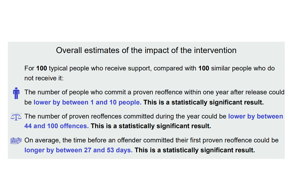
Contains a series of statements on what you can and cannot say about the one-year reoffending rate; about the one-year reoffending frequency and about the time to first reoffence

Source: Ministry of Justice (2020)

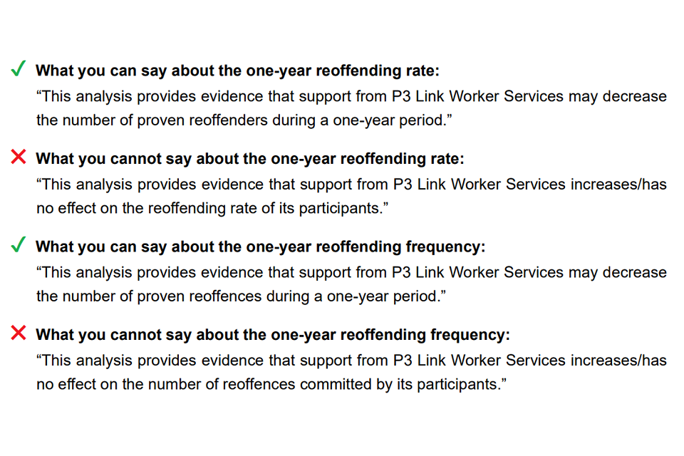
Source: Ministry of Justice (2020)

Summary charts

these show two of the outcomes measures presented graphically, with confidence intervals also shown (see Figure 2 for an example).

Figure 2 Summary charts

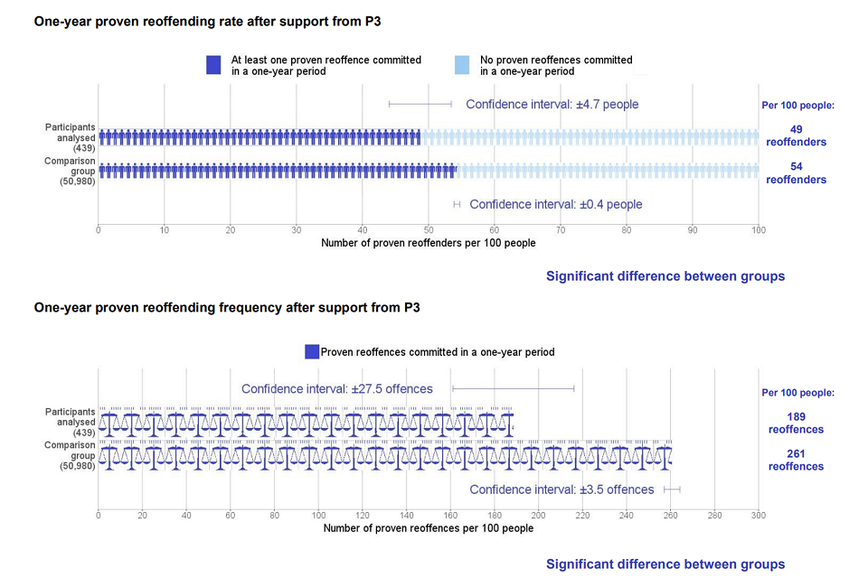
Source: Ministry of Justice (2020)

‘Intervention’ in their own words

This is a short description of the intervention in the words of the organisation delivering the intervention

Response from “organisation” to the Justice Data Lab analysis

This is the reaction of the delivery organisation to the results of the analysis

Results in detail

This briefly explains the geographic coverage of the intervention across each of the different outcome measures
Statistically significant results are described alongside the table of results (see Figure 3 for an example)

Figure 3 Results in detail

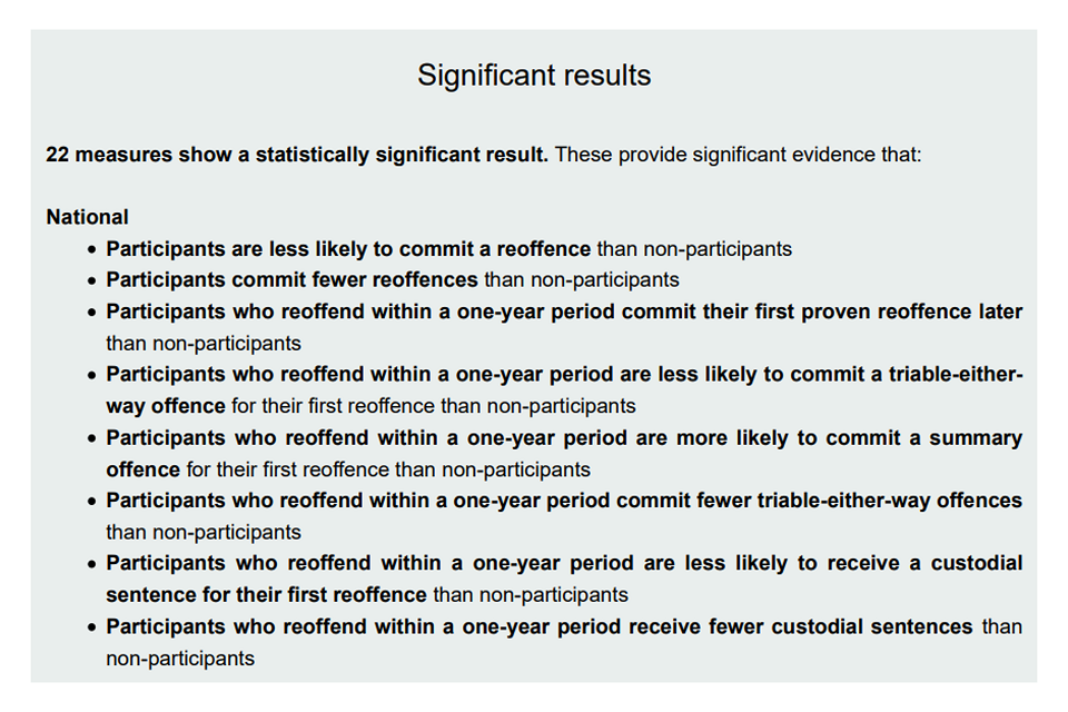
Source: Ministry of Justice (2020)

Source: Ministry of Justice (2020)

Profile of the treatment group

This section details the profile of the treatment group showing those who are, and are not, included in the analysis (see Figure 4 for an example)

Figure 4 Profile of the treatment group

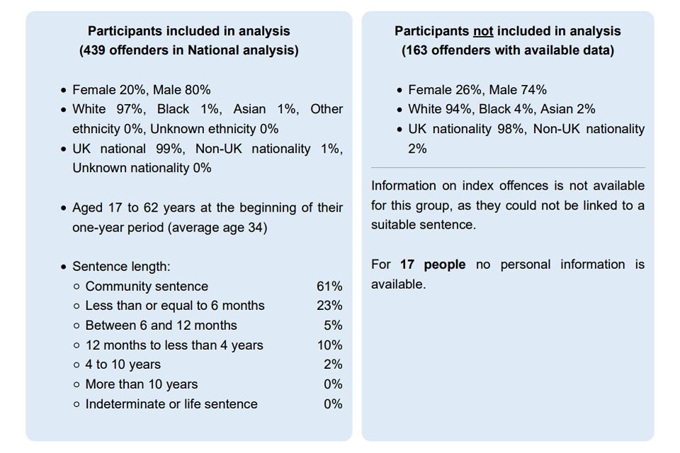
Source: Ministry of Justice (2020)

Matching the treatment and comparison groups

This is a short description of the matching quality for each geographical analysis (with more details provided in an annex)

Numbers of people in the treatment and comparison groups

The reports conclude with a flow diagram showing why some participants were excluded from the analysis (example shown in Figure 5)

Figure 5 Numbers of people in the treatment and comparison groups [Exert of full diagram]

Source: Ministry of Justice (2020)

3.4 Implications for the Employment Data Lab

The review of past evaluations of active labour market programmes highlights the need for the Employment Data Lab to carry out a number of tasks before commencing each evaluation. Firstly, it is necessary to identify the objectives of the intervention and who it seeks to help. This should include the eligibility criteria that individuals are expected to meet in order to take part, the proportion of those meeting the eligibility criteria who participate in the programme, as well as the number, and where the intervention is running^{[footnote 8]}. The initial phase of work should also identify when the intervention started and the length of time support will be offered to participants. Depending on the scale of the intervention, it may be immediately apparent that a causal impact estimate is unlikely to be possible, or that particular methods of identifying causal impact are more likely to detect any impact than others.

As well as understanding the nature of the intervention and the eligible population, it is necessary to decide on an appropriate set of outcome measures which are expected to be affected by the intervention. These would ideally distinguish between one or two primary outcomes, where an impact would be seen if the programme is effective, and any other secondary outcomes. The way in which outcome measures are defined should take into account the likely time-period over which impacts are expected to be seen and what can be observed in the available data. It is also important to consider whether any other policy changes may have affected the outcome measures over the period of time to be considered in the analysis.

Having extracted the basic information on the intervention, this can be used to decide on the most appropriate way of estimating impact. PSM has been widely used in past evaluations of active labour market programmes where participation is voluntary and is most likely to be suited to the work of the Employment Data Lab. Having access to linked administrative data increases the likelihood that the requirement that the treatment and comparison groups are matched on all characteristics likely to influence the probability of treatment and outcomes will be satisfied. It is also more likely to be possible to identify a well-matched comparison group with the large sample sizes that access to administrative data provides.

The fact that the approach has been frequently used in past evaluations based on DWP and HMRC administrative data means that it is possible to draw on existing evidence which can be used to inform the choice of matching variables. The linked data available through the Employment Data Lab also has the advantage of spanning a long period of time, and so, depending on the nature of the intervention, it may be possible to combine PSM with DiD analysis, as has been the case in many past studies of active labour market programmes. DiD methods are widely used in evaluation of area-based interventions in particular, but as participation in the interventions to be evaluated by the Employment Data Lab is voluntary, DiD is likely to be less useful as a technique to be deployed independently of PSM.

From the review of previous evaluations of active labour market programmes using PSM it is apparent that it is important to report on the balance between the treatment and comparison groups after matching to demonstrate that the process is effective in ensuring that the matched comparison group are similar to the treatment group on the characteristics which are likely to affect outcomes. This includes showing the mean standardised bias and whether any outstanding differences in characteristics between the treatment group and the matched comparison group are statistically significant as well as general measures of balance such as Rubin’s B and Rubin’s R. It is also necessary to consider whether the findings are likely to reflect the impact of the intervention on all treated individuals, or only a subset by reporting the percentage on (or off) support. Finally, exploring whether the findings vary when different matching algorithms are used provides an insight into the robustness of the impact estimates.

CEM is a fairly recent development in evaluation methodology, but there are examples of it being used in evaluations of active labour market programmes. It can be more feasible to implement than PSM when the treatment and comparison groups are large. However, as many of the interventions that are likely to be evaluated by the Employment Data lab are relatively small in scale, it may be of less relevance than other more established techniques.

Duration analysis can be used to estimate the impact of programmes which are rolled out to an existing stock of claimants in circumstances where it is not possible to offer the intervention to all individuals at once. There are many examples of its application to the evaluation of active labour market programmes when this is the case. However, it is also only applicable when the aim is to move participants from one state to another, so it is not suited to estimating the impact of the intervention on a wide range of different types of outcomes.

A RDD is only feasible in circumstances where there is a threshold for treatment and it is also possible to observe whether individuals fall just above or below threshold for treatment, based on objective criteria. Whilst this is possible for some active labour market programmes, it is often not the case. It also has the limitation of only estimating the impact of the intervention at the margin of treatment, rather than the average treatment effect across all treated individuals. It is unlikely to be of general use to the Employment Data Lab except perhaps in the case of interventions where access is limited to those within a particular age bracket.

Instrumental variables analysis has been used in some past evaluations of active labour market programmes, but the difficulties inherent in finding a suitable instrument mean that it is unlikely to be possible to implement this approach within the Employment Data Lab. It is necessary to have a detailed knowledge of the context within which the intervention is implemented to establish whether there is likely to be a suitable instrument and the administrative data may not contain suitable instruments in many cases.

There are many aspects of the approach taken by the Justice Data Lab that the Employment Data Lab could usefully replicate. For example, it demonstrates the need to provide clear information to delivery organisations on the aims of the Lab, how it works and the value to delivery organisations of allowing their interventions to be evaluated. It also provides an overview of the sort of information that is needed from delivery organisations in order to carry out an evaluation, including the minimum number of programme participants, and a standardised template that could potentially be adapted to the needs of the Employment Data Lab. It would be helpful for the Employment Data Lab to consider from the outset whether it is possible to work within existing data protection legislation to improve the likelihood of being able to carry out future meta analyses of similar interventions to increase knowledge on effective programmes.

Other lessons learned from the Justice Data Lab are the need to identify a set of outcome measures which are likely to be appropriate to judging the impact of the types of interventions the Employment Data Lab will evaluate. Ideally these outcome measures should be universally accepted by delivery organisations as relevant to what they are trying to achieve. Focusing on a limited number of outcomes is likely to aid comparability between evaluations of different programmes and increase the contribution that the Employment Data Lab can make to understanding of the types of interventions which are most effective. Identifying at least some outcome measures which are likely to capture impacts fairly soon after participation in the intervention is also important to ensure that any impacts can be attributed to the programme rather than other changes that occur over time.

As well as identifying a suitable range of outcome measures, the Justice Data Lab highlights the need to draw up a list of matching variables. This should be appropriate to ensuring that treatment and comparison groups are well-matched across the range of characteristics which are likely to determine whether they participate in an intervention, as well as their likelihood of attaining each of the main outcomes.

The Employment Data Lab could usefully learn from some of the criticism of the Justice Data Lab by placing greater weight on the quality of the match between treatment and comparison groups. For example, as well as reporting on a wider range of measures to assess the quality of the match, it would be advisable for the Employment Data Lab to base the selection of matching variables on existing evidence on the determinants of programme participation, rather than a standardised approach to reducing the number of matching variables. It would also be useful to consider whether there are any characteristics which members of the treatment and comparison groups should be hard-matched on, such as gender.

The approach to reporting used by the Justice Data Lab has a focus on clear, accurate and visual reporting which includes caveats and provides guidance on interpretation. The Employment Data Lab could certainly benefit from taking a similar approach, but it would be useful to include more checks on the robustness of the impact estimates. This could include testing the sensitivity of the findings to the use of different matching estimators. Also, to reduce the potential for criticism of methodological choices it would be helpful to provide a detailed explanation of the reasons for particular analytical decisions and to also acknowledge areas where there is a lack of evidence to inform these decisions.

Question 5

4 Review  of selected approaches

Accepted Answer

4.1 Introduction

This chapter provides a detailed description of the main considerations when implementing PSM, as the quasi-experimental method most likely to be suited to the work of the Employment Data Lab. This draws on a review of the relevant literature. It also explains how the approach can be implemented in software packages currently available to the Employment Data Lab team. It also outlines the potential to use machine learning in future programme evaluations and proposes this as an area for future development.

4.2 Propensity Score Matching

This section sets out the main analytical decisions when implementing PSM. A number of papers provide a detailed description of the steps required to carry out PSM, including Caliendo and Kopeinig (2008). Having decided whether the approach is appropriate by considering whether the assumptions set out in section 2.3.1 are likely to be met, it is necessary to decide on the choice of matching estimator. This is the algorithm used to identify a well-matched comparison group. Section 4.2.1 provides details of the different approaches to matching and current thinking on each^{[footnote 9]}. Section 4.2.2 then moves on to explain how the quality of the match between the treatment and comparison groups can be explored. The section concludes by setting out a number of different approaches to assessing the likelihood that the impact estimates are robust.

4.2.1 Matching estimators

Nearest Neighbour

The simplest and most intuitive matching estimator involves nearest neighbour matching. This is where a member of the treatment group is matched to the individual from the comparison group with the most similar propensity score. Where one treated individual is matched to a single individual from the comparison group this is known as one-to-one matching. As well as one-to-one matching, it is possible to match each member of the treatment group to a number of comparators with a similar propensity score. This is known as one-to-many matching or over-sampling (Caliendo and Kopeinig 2008, 9). Two other variants of nearest neighbour matching are possible:

matching with replacement means an untreated individual can be used multiple times as a match if they are the closest available match for more than one member of the treatment group
matching without replacement means that each potential comparator can be used only once. The impact estimates will depend on the order in which observations are matched as the number of potential comparators with similar propensity scores will fall with each successive match. It is therefore important to ensure that the order in which members of the treatment group are matched is random to avoid bias in the impact estimate

Matching with replacement can make it easier to find close matches between the treatment and comparison groups when the size of the comparison group is limited relative to the size of the treatment group, and/or there is limited overlap in the propensity scores of the two groups. For example, if a large proportion of the treatment group have high propensity scores but there are only a few potential comparators with high propensity scores, matching with replacement would reduce the likelihood of high-scoring participants being matched to low-scoring non-participants. This would increase the likelihood of impact estimates being robust as outcomes for the matched comparators would be likely to provide a more reliable estimate of the counterfactual than if matching without replacement was used.

Whilst matching with replacement offers benefits in terms of reducing the number of non-participants required to estimate counterfactual outcomes compared to matching without replacement, it has the disadvantage of increasing the variance, meaning that impact estimates less likely to be statistically significant (Caliendo and Kopeinig 2008). This is also the case with matching to more than one nearest neighbour, as whilst this reduces the variance, it may also increase the risk of bias as some of the matches may be weaker. Setting a threshold for the maximum number of matches appropriate to the distribution of propensity scores and the number of times each member of the control group is likely to be matched, as well as applying a weight to comparators which reflects the closeness of the match to the member of the treatment group can help to reduce the risk of bias (Stuart 2010).

Due to the weaknesses with each approach to nearest neighbour matching, described above, it has been largely superseded by more sophisticated matching estimators.

Calliper

Calliper matching involves finding a single match for a treated individual from members of the comparison group with a propensity score within a specified range or tolerance level of that of the treated individual (known as the calliper). It has the advantage over nearest neighbour matching of preventing treated individuals being matched to comparators with a very different propensity score, purely because they are the nearest match.

A tighter calliper means that the matched comparison group will be a closer match for the treatment group than where the calliper is wider. With a tighter calliper, the estimate of the counterfactual is more likely to reflect the outcomes that the treatment group would have experienced if they had not received the intervention. However, as with all matching estimators, requiring a close match can reduce the likelihood of finding comparators for all members of the treatment group, and so the impact estimate may only be representative of the impact of the intervention on a subset of participants i.e. the percentage off support may be higher. The requirement that the matched comparator must have a propensity score within a given range of the treated individual increases the likelihood that treated individuals will be off support compared with nearest neighbour matching.

The reliability of impact estimates produced using calliper matching depends in part on whether the chosen calliper is appropriate. As it is difficult to know prior to undertaking calliper matching what level of tolerance is ideal, sensitivity checks to varying this are required when undertaking calliper matching.

Radius

Radius matching is a variant of calliper matching. With this approach, a treated individual is matched to all comparators with a propensity score within a given radius, rather than the single individual with the most similar propensity score within that range. It offers greater flexibility over the selection of matched comparators than nearest neighbour matching, as it is less reliant on using information from a specific number of matches. Rather, it makes use of information from all matches where many close matches are available whilst limiting the number of comparators to maintain the quality of the match where few members of the comparison group have a similar propensity score. However, as with calliper matching, radius matching will only produce a reliable estimate of impact if a suitable radius is chosen and deciding on an appropriate radius can be difficult.

Stratification

Stratification matching subdivides the treatment and comparison groups into a series of strata. Each block covers a specified range of propensity scores and individuals in the treatment and comparison groups with scores in this range are matched (Becker and Ichino 2002). When correctly defined, the approach to defining the strata ensures that the covariates are balanced and the assignment to the treatment can be considered random.

With stratification matching, the impact of the intervention is calculated by taking the mean difference in outcomes between the treatment and comparison groups within each stratum. The average treatment effect is weighted by the distribution of treated units across the strata. This method is also referred to as interval matching, blocking or subclassification.

Previous research suggests that having five strata is adequate to remove 95 per cent of the bias associated with differences in covariates (Imbens 2004). Checking the balance between the treatment and comparison groups on the propensity score or covariates within each stratum provides a check that the number of strata selected is appropriate. If within a stratum the treatment and comparison groups are not balanced on the propensity score, the strata are too large and need to be split.

Kernel

Kernel matching involves using a weighted average of individuals in the comparison group to estimate the counterfactual. Comparators with the most similar propensity score to the treated individual will receive the highest weight. As information on multiple members of the comparison group is potentially used, this can reduce the variance. Set against this, there is a risk that impact estimates are biased by the inclusion of weaker matches.

The weights used in kernel matching depend on the difference in propensity scores between treated and untreated individuals. It is necessary to choose between different types of kernels and select an appropriate bandwidth. Bandwidths will be discussed in more detail in the next section.

Local Linear Regression

Like kernel matching, local linear regression matching is a non-parametric matching estimator. The main difference between kernel and LLR matching is that with LLR the weighted regression underlying the approach includes a linear term. A LLR approach is preferable to kernel matching in cases where comparison group observations are distributed asymmetrically around the treatment group observations or when there are gaps in the propensity score distribution.

Figure 6 A comparison of PSM matching estimators

Estimator	Advantages	Disadvantages
Nearest Neighbour	Relatively simple to implement and explain. Can use either one-to-one matching or one-to-many matching, with or without replacement.	The order in which cases are matched without replacement may affect the size of the impact estimates. Matching with replacement increases the variance, reducing the likelihood of detecting any impacts.
Calliper	Prevents treated individuals being matched to comparators with a very different propensity score.	Impact estimates may vary with calliper choice and appropriate calliper may be difficult to determine.
Radius	Makes use of information from all matches where many close matches are available.	Radius matching will only produce a reliable estimate of impact if a suitable radius is chosen.
Stratification matching	When correctly defined, the approach to defining the strata ensures that the covariates are balanced and the assignment to the treatment can be considered as good as random.	If within a stratum the treatment and comparison groups are not balanced on the propensity score, the impact estimates may be unreliable.
Kernel	As information on multiple members of the comparison group is potentially used, this can reduce the variance.	Impact estimates may be biased by the inclusion of weaker matches.
Local linear regression	Preferable to kernel matching when comparison observations are distributed asymmetrically around the treatment observations or when there are gaps in the propensity score distribution.

4.2.2 Balance between the treatment and comparison groups

As is apparent from the previous section, as well as giving careful consideration to the choice of matching estimator, it is important to assess how well the matched comparison group is likely to represent the counterfactual. This includes checking the balance on covariates between the treatment and matched comparison group and how varying the choice of matching estimator affects the results. This subsection covers ways of assessing the quality of the match and the robustness of the evaluation findings.

Covariate balancing

A simple way of determining how likely the matched comparison group is to provide a robust estimate of the counterfactual is to compare the characteristics of the treatment group with those of the unmatched and matched comparison groups. This provides an insight into how well the matching process adjusts the characteristics of the comparison group to mimic those of the treatment group. If sizeable differences between the two groups remain across a range of characteristics following matching, this suggests that PSM is unlikely to provide an accurate estimate of the impact of the intervention. Again, it is important to note that even if the treatment group is well-matched to the comparison group on observed characteristics, the impact estimate may be unreliable if there are differences between the two groups in unobserved characteristics which determine the likelihood of being treated and outcomes.

As well as reporting the proportion of the treatment, unmatched comparison group and matched comparison group with a given characteristic, it is common to assess the statistical significance of any apparent differences in characteristics between the treatment and matched comparison groups using the Mean Standardised Bias (MSB). The MSB is calculated by dividing the difference in means between the treatment and matched comparison groups on each of the matching variables by the square root of the mean sample variance. This is expressed as a percentage. As with a t-test, with a large sample the MSB can appear statistically significant even when it is small and so it is usual to take into account both the size of the MSB and whether it is statistically significant. An MSB in excess of 5 per cent suggests greater reason to be concerned about imbalance between the treatment and matched comparison groups.

Visual ways of assessing balance include examining box plots or quantile–quantile (Q-Q) plots to compare the distribution of variables between the treatment and comparison groups (Imai, King, and Stuart 2008; Stuart 2010).

Rubin’s B and R

Rubin’s B and Rubin’s R are summary measures of the balance between the treatment and matched comparison groups across all covariates. Rubin’s B is the absolute standardised difference of the means of the propensity score in the treatment and matched comparison groups. Rubin’s R is the ratio of the treatment to matched comparison group variances in the propensity scores. Rubin (2001) suggests that, for the two groups to be well-matched, the value of B should be less than 25, whilst R should lie between 0.5 and 2.

In combination, Rubin’s B and Rubin’s R are informative in considering the trade-off between bias and variance between the treatment and matched comparison groups. In Stata (a statistical software package) the statistics can be calculated using the pstest ado file.

Percentage off support and Lechner Bounds

As mentioned previously, the percentage off support is the percentage of the treatment group for whom no suitable comparators exist. It is calculated by dividing the number off support (those for whom there is no comparison group match) divided by the total number in the treatment group. These numbers are reported in the psmatch2 package in Stata.

A high percentage off support indicates that the impact estimates are not representative of the impact of the intervention across all treated individuals, whereas the percentage off support may be low if the treatment and comparison groups are not closely matched.

Lechner (2000) proposes a way of using information on members of the treatment group who cannot be matched to the comparison group to calculate non-parametric bounds of the parameter of interest if all treated individuals had been included. He suggests routinely carrying out this analysis to assess the sensitivity of impact estimates to focusing on a subset of the treatment group.

Entropy Balancing

Ideally the choice of matching variables when using PSM should be based on existing knowledge about the likely drivers of outcomes as well as the factors which determine whether an individual participates in an intervention. However, in practice it is common for knowledge to be patchy. As a result, it is common for analysts to re-estimate propensity scores with different sets of matching variables to seek to improve the balance between the treatment and comparison groups. However, there is no straightforward way of ensuring that this process improves the balance between the treatment and comparison groups (Iacus, King, and Porro 2012).

Entropy balancing addresses these shortcomings and uses a pre-processing scheme where covariate balance is directly built into the weight function that is used to adjust the comparison group to replicate the characteristics of the treatment group (Hainmueller 2012). It thus reduces the need for experimentation when implementing PSM.

One of the properties of entropy balancing is that it always improves on the covariate balance achieved by conventional pre-processing methods. Balance checking is therefore no longer needed. Another advantage is that the weights commonly retain more information than some other approaches, such as nearest neighbour matching. Entropy balancing can be combined with other matching methods and the resulting weights are compatible with many standard estimators for subsequent analysis of the reweighted data. It can be implemented in Stata using the ebalance package (devised by Hainmueller and Xu (2013)), but as yet has been little used in the evaluation of active labour market programmes. Examples include studies of the short- and long-run effects of decentralising public employment services on job placements (Weber 2016) and an evaluation of the effect of work-related training on social capital and earnings, both based on analysis of German data (Ruhose, Thomsen, and Weilage 2019).

Covariate balancing propensity score weighting

Like entropy balancing the covariate balancing propensity score (CBPS) technique seeks to reduce the difficulties inherent in balancing the characteristics of treatment and comparison groups (Imai and Ratkovic 2014). It aims to model assignment to the treatment group whilst also optimising the balance on covariates by exploiting the dual characteristics of the propensity score as a covariate balancing score and the conditional probability of treatment assignment. Unlike the entropy balancing method, CBPS constructs balancing weights directly from the propensity score. Again, as a newer technique, it is more experimental and has not been widely implemented at this point in time. However, it can be implemented using the Stata psweight ado command.

The psweight command can also be used to compute inverse probability weights based on logistic regression. These can be used to estimate the average treatment effect, the average treatment effect on the treated and the average treatment effect on the untreated.

4.2.3 Sensitivity testing

Choosing an appropriate bandwidth

The closeness of the match between the treatment and comparison groups is fundamental to whether PSM provides a reliable estimate of the counterfactual. As is apparent from the earlier sections, choosing an appropriate bandwidth is crucial as a wider bandwidth will increase the likelihood of finding matches for members of the treatment group, but at the cost of the matches being less close. A wider bandwidth increases the likelihood of bias in the impact estimator, but a higher number of comparators will reduce the variance around point estimates. Selecting an appropriate calliper or bandwidth is therefore essential in producing accurate impact estimates and reaching the correct conclusions about the impact of an intervention (Galdo, Smith, and Black 2008).

Despite the importance of selecting the correct bandwidth to devising a reliable estimate of impact when using PSM, there is no natural default when selecting the bandwidth, or a method of calculating the optimal bandwidth which is appropriate to all circumstances (Busso, DiNardo, and McCrary 2014). Indeed, as Li (2012) emphasizes, little is known about the optimal bandwidth, radius, and ideal number of matches. One approach is to use data driven methods, such as the mean integrated squared error (MISE) or Silverman’s Rule of Thumb to choose these parameters (Galdo, Smith, and Black 2008; Silverman 1986). However, Silverman’s Rule of Thumb^{[footnote 10]} only provides a good guide to bandwidth if the propensity score follows the normal distribution (Härdle et al. 2012).

Rosenbaum Bounds

Rosenbaum (2002) distinguishes between overt and hidden biases in observational studies. An overt bias can be seen in the data prior to treatment. For example, the treatment group may be older than the comparison group. Alternatively, bias may be hidden because information is unobserved or unrecorded. Whilst it may be possible to adjust for overt biases using techniques such as matching, hidden bias can undermine the robustness of the analysis as unobserved variables may affect assignment to the treatment group or affect outcomes. Where eligible individuals are able to choose whether to participate in an intervention, motivation is often cited as an unobserved characteristic which can affect both the likelihood of participation and the outcomes that the individual attains as a result of participation. If outcomes for highly motivated individuals who choose to take part in an intervention are compared against those for less motivated individuals who do not wish to participate, this is likely to result in an upward bias in the estimate of impact.

Rosenbaum bounds provides an indication of the likelihood that results may be invalidated by hidden bias. The Stata mhbounds package developed by Becker and Caliendo (2007) implements Rosenbaum bounds for binary outcome variables, such as employment or unemployment, using the Mantel-Haenszel statistic whilst rbounds, developed by DiPrete and Gangl (2004) test sensitivity for continuous outcome variables. A further development is rmhbounds, developed by Litwok (2020). This seeks to address some of the limitations of mhbounds which means it is only suited to some types of matching estimator.

4.3 Machine Learning

Machine learning can be used to find patterns in data and is potentially helpful in the field of programme evaluation because it can make it possible to identify relationships which might otherwise not be apparent to researchers. For example, Goller et al. (2020) suggest that machine learning can be useful when estimating propensity scores because it can help identify variables that are important in determining who is treated. Provided these variables are included in the data available to researchers, machine learning can be used to detect the important variables and reduce the risk of omitted variable bias. For example, sensimatch is a new Stata package which can be used to choose between large numbers of potential matching variables. It is based on a machine learning approach and works by excluding variables at random until the optimal set is chosen (Cerulli 2019).

Athey and Imbens (2017) give an overview of the relative strengths and weaknesses of machine learning techniques in a range of applications and provides a good introduction to the topic. Knaus, Lechner and Strittmatter (2020) compare the consistency of findings across a range of different machine learning algorithms when estimating the impact of job search programmes in Switzerland using social security data. They conclude that random forest-based estimation approaches offer the best overall performance. The approach builds on the causal tree, where a sample is split multiple times into ever smaller strata. These groups become increasingly homogenous until some stopping criterion is reached. At this point, the treatment effect can be computed within each stratum as the difference in mean outcomes between the treatment and comparison group. The random forest estimator averages the prediction across many trees by generating random subsamples and making the splitting decision based on a random selection of covariates (Bart Cockx, Lechner, and Bollens 2019).

Cockx et al. (2019) use a variant of the random forest-based estimation approach known as Modified Causal Forests to evaluate differences in the effectiveness of three different types of training programmes for particular groups of unemployed job seekers in Flanders. The analysis is based on administrative data and provides a detailed description of machine learning methods. Goller et al. (2020) also provides a useful example of using machine learning in estimating the propensity score to evaluate programmes for the long-term unemployed in Germany.

Question 6

5 Conclusions  and recommendations

Accepted Answer

5.1 Introduction

This chapter sets out a proposed methodology for the Employment Data Lab, based on the findings arising from the literature reviewed in the earlier chapters. It also summarises how these approaches can be implemented.

5.2 Proposed methodology for the DWP Employment Data Lab

The review of evaluations of active labour market policies in Chapter 3 provides a list of outcome measures used in past studies of the sorts of interventions that the Employment Data Lab is likely to evaluate. It would be helpful for the Employment Data Lab to draw up a comprehensive list of outcome measures that could be observed within the available data. These should be focused on data items that are known to be recorded to a high degree of accuracy and to span the range of the different types of interventions that are likely to be assessed by the Lab.

Prior to submitting data on programme participants for evaluation, organisations delivering interventions should be asked to provide some basic information on the nature of the intervention, its aims and those targeted by the intervention. This should include the following topics:

A brief description of the intervention
Details of any eligibility criteria that individuals have to meet before they are able to receive the intervention
Any other restrictions on eligibility, such as whether the programme is only available in particular areas
The numbers of individuals who have received support. Ideally this would be a detailed breakdown by month
The number of treated individuals where a national insurance number is recorded
Identifying one or two primary outcomes expected to be affected by the intervention, from the list supplied by the Employment Data Lab
Specifying any secondary outcomes likely to be affected (again drawing from the Employment Data Lab list)
The timeframe over which any short- medium and longer-term impacts are expected to be seen if the programme is effective

Having obtained this preliminary information from programme providers, it should be possible to assess the likelihood of being able to estimate the impact of the intervention or whether an evaluation is likely to be possible at a later point in time.

The review of active labour market programmes suggests that PSM is most likely to be suited to evaluating the impact of interventions where participation is voluntary provided the linked administrative data is sufficiently rich to be able to observe the full range of factors likely to affect whether an individual participates in the programme as well as the outcomes they are likely to attain. Whether this is credible will depend in part on the nature of the intervention and the eligibility criteria, but the level of detail available in the linked data means there is a reasonable chance of being able to satisfy the assumptions underlying PSM. This could be further enhanced in the future by continuing to pursue linking to a wider range of datasets to improve the range of available matching variables.

The fact that the linked administrative data can potentially provide access to large numbers of comparators is a strength when it comes to PSM, and as the data spans many years in some cases it may be feasible to combine PSM with DiD. This may be of value in cases where the available matching variables are insufficient to adjust for differences in unobservable characteristics between the treatment and comparison groups which might affect outcomes, but which are likely to be constant over time.

Many of the interventions to be evaluated by the Employment Data Lab are relatively small in scale. For example, a survey of organisations delivering programmes which could potentially be evaluated by the Employment Data Lab found that interventions most commonly had between 101 and 200 participants over the course of a year. PSM is well-suited to evaluating the impact of small-scale interventions, so it is recommended that in the short-term this should be the priority.

Once the Employment Data Lab has achieved basic functionality, focused around implementing the PSM approach, there would be some value in expanding the range of evaluation techniques. This would make it possible to evaluate the impact of a wider range of interventions. For example, the survey of interventions carried out by the Employment Data Lab found that more than one-in-10 programmes (10.8 per cent) had over 5,000 participants over the course of a year. It would potentially be time-consuming to identify matches using PSM when the treatment group is very large, so CEM may be better suited to estimating the impact of some of the large-scale programmes evaluated by the Employment Data Lab.

As noted in Chapter 3, whilst some other evaluation methods may be less generally applicable than PSM, they may make it possible to estimate impact in circumstances where PSM is not feasible. Depending on the future remit and resourcing of the Employment Data Lab, a wider range of methods such as RDD and duration analysis may be relevant. However, arguably a stronger priority for future development is machine learning. This could be used to assist in the selection of matching variables when implementing PSM and to test the sensitivity of the impact estimates to using different ways of estimating the counterfactual.

5.3 Implementation

This section provides a summary of the steps required to implement the recommendations set out in the previous section. It also refers to available Stata software packages which can be used to carry out particular tasks.

Step 1 – Draw up list of outcome measures

Step 2 – Devise a list of questions for programme providers

Step 3 – Draw up a list of potential matching variables from past evaluations which have been based on DWP and HMRC administrative data

This could be used to identify core matching variables and those which are relevant to estimating the impact of particular types of interventions.

Step 4 – Implement PSM using pstest and psmatch2

This should include assessing the balance between the treatment and matching comparison groups on individual matching variables (using mean standardised bias) and Rubin’s R and B, as well as computing the percentage on support. The analysis should explore the sensitivity of the findings to varying the choice of matching estimators and the closeness of the match e.g. by varying the bandwidth and calculating Rosenbaum Bounds to assess the likelihood that the results could be invalidated by hidden bias. This could be done using rmhbounds for binary outcome variables or rbounds for continuous outcome variables.

Step 5 – Having achieved basic functionality, the recommended priorities for future development are:

experimenting with approaches designed to assist in balancing the characteristics of the treatment and comparison groups and in the selection of matching variables, such as entropy balancing (using ebalance), covariate balancing propensity score weighting (using psweight) and machine learning (using sensimatch)
using machine learning approaches to assess the robustness of the findings to alternative methods of estimating impact
applying CEM to estimate the impact of programmes where the treatment group is very large (using the cem package)
increasing the range and complexity of evaluation techniques to expand the types of interventions which could be evaluated by the Employment Data Lab

These areas for future development are listed in rough order of priority. A further option would be to explore the feasibility of giving external organisations access to the data to carry out their own independent evaluations. This would reduce the likelihood that capacity constraints limit the ability of the Employment Data Lab to produce timely and robust evidence. It would also help to build knowledge and skills in working with the data and applying evaluation methods to linked administrative datasets. This may be the most efficient way of increasing the capacity of the Employment Data Lab to apply a wider range of techniques to evaluate the effectiveness of a diverse range of programmes. It could also be used to build a community of expert users, providing peer review and quality assurance of outputs.

Question 7

6 Bibliography

Accepted Answer

Abadie, A., Drukker, D., Herr, J.L. and Imbens, G.W. (2004) Implementing matching estimators for average treatment effects in Stata. The Stata Journal, 4(3), pp.290–311.

Alegre, M.A., Casado, D., Sanz, J. and Todeschini, F.A. (2015) The impact of training‐intensive labour market policies on labour and educational prospects of NEETs: evidence from Catalonia (Spain). Educational Research 57: 151–167.

Arellano, A. F. (2010) Do training programmes get the unemployed back to work? A look at the Spanish experience. Revista de Economía Aplicada 18: 39–65.

Athey, S. (2017) Beyond prediction: Using big data for policy problems. Science, 355(6324), pp.483–485.

Athey, S. and Imbens, G.W. (2017) The state of applied econometrics: Causality and policy evaluation. Journal of Economic Perspectives, 31(2), pp.3–32.

Austin, P.C. (2011) Optimal caliper widths for propensity‐score matching when estimating differences in means and differences in proportions in observational studies. Pharmaceutical statistics, 10(2), pp.150–161.

Autor, D.H. and Houseman, S.N. (2010) Do temporary‐help jobs improve labor market outcomes for low‐skilled workers? Evidence from “Work First”. American Economic Journal: Applied Economics 2: 96–128.

Autor, D.H., Houseman, S.N. and Pekkala Kerr, S. (2017) The effect of work first job placements on the distribution of earnings: an instrumental variable quantile regression approach. Journal of Labor Economics 35: 149–190.

Baumgartner, H.J. and Caliendo, M. (2008) Turning unemployment into self‐employment: effectiveness of two start‐up programmes. Oxford Bulletin of Economics and Statistics 70: 347–373.

Becker, S.O. and Caliendo, M. (2006) mhbounds-Sensitivity Analysis for Average Treatment Effects. Software.

Becker, S.O. and Caliendo, M. (2007) Sensitivity analysis for average treatment effects. The Stata Journal, 7(1), pp.71–83.

Bergemann, A., Fitzenberger, B. and Speckesser, S. (2009) Evaluating the dynamic employment effects of training programs in East Germany using conditional difference‐in‐differences. Journal of Applied Econometrics 24: 797–823.

Bewley, H. (2012) The effectiveness of different community order requirements for offenders who received an OASys assessment. Ministry of Justice Research Series 17/12.

Bewley, H. Dorsett, R. and Haile, G. (2007) The Impact of Pathways to Work, Research Report 435. Leeds: DWP.

Bewley, H., Dorsett, R. and Ratto, M. (2008) Evidence on the effect of Pathways to Work on existing claimants, Research Report 488. Norwich: DWP.

Bewley, H., Dorsett, R. and Salis, S. (2008) The impact of Pathways on benefit receipt in the expansion areas, Research Report 552. Norwich: DWP.

Bewley, H., Dorsett, R. and Salis, S. (2009) The impact of Pathways to Work on work, earnings and self-reported health in the April 2006 expansion areas. Department for Work and Pensions Research Report 601. Norwich: DWP.

Blackwell, M., Iacus, S., King, G. and Porro, G. (2009) CEM: Coarsened exact matching in Stata. The Stata Journal, 9(4), pp.524-546.

Blien, U. and Caliendo, M. (2009) Startup subsidies in East Germany: finally, a policy that works? International Journal of Manpower 30: 625–647.

Brock, T. and Harknett, K. (1998) A comparison of two welfare–to‐work case management models. Social Service Review 72: 493–520.

Busso, M., DiNardo, J. and McCrary, J., 2014. New evidence on the finite sample properties of propensity score reweighting and matching estimators. Review of Economics and Statistics, 96(5), pp.885–897.

Caliendo, M. and Kopeinig, S., 2008. Some practical guidance for the implementation of propensity score matching. Journal of economic surveys, 22(1), pp.31–72.

Caliendo, M. and Künn, S. (2011) Start‐up subsidies for the unemployed: long‐term evidence and effect heterogeneity. Journal of Public Economics 95: 311–331.

Caliendo, M., Künn, S. and Mahlstedt, R. (2017) The return to labor market mobility: an evaluation of relocation assistance for the unemployed. Journal of Public Economics 148: 136–151.

Capuano, S., Cockett, J., Gray, H. and Papoutsaki, D. (2019) ‘The impact of the minimum wage on employment and hours.’ Institute for Employment Studies Research Report 538. Low Pay Commission. December 2019.

Card, D., Kluve, J.,Weber, A., What Works? A Meta-Analysis of Recent Active Labor Market Program Evaluations, Journal of the European Economic Association, Volume 16, Issue 3, June 2018, Pages 894–931, https://doi.org/10.1093/jeea/jvx028

Centeno, L., Centeno, M. and Novo, A.A. (2009) Evaluating job‐search programs for old and young individuals: heterogeneous impact on unemployment duration. Labour Economics 16: 12–25.

Cerqua, A., Urwin, P., Thomson, D. and Bibby, D., 2020. Evaluation of education and training impacts for the unemployed: Challenges of new data. Labour Economics, 67, p.101907.

Cerulli, G., 2019. Data-driven sensitivity analysis for matching estimators. Economics Letters, 185, p.108749.

Cockx, B. and Dejemeppe, M. (2007). ‘Is the notification of monitoring a threat to the unemployed? A regression discontinuity approach’, IZA Discussion Paper No. 2854.

Diamond, A. and Sekhon, J.S., 2013. Genetic matching for estimating causal effects: A general multivariate matching method for achieving balance in observational studies. Review of Economics and Statistics, 95(3), pp.932–945.

DiPrete, T.A. and Gangl, M., 2004. 7. Assessing bias in the estimation of causal effects: Rosenbaum bounds on matching estimators and instrumental variables estimation with imperfect instruments. Sociological methodology, 34(1), pp.271–310.

Dorsett, R. (2006) The New Deal for Young People: effect on the labour market status of young men. Labour Economics 13: 405–422.

Dorsett, R., Gray, H., Speckesser, S. and Stokes, L. (2019) ‘Estimating the impact of Traineeships’. Research Report 919. Department for Education.

Dorsett, R., Smeaton, D. and Speckesser, S. (2013) The effect of making a voluntary labour market programme compulsory: evidence from a UK experiment. Fiscal Studies 34: 467–489.

Fitzenberger, B., Orlanski, O., Osikominu, A. and Paul, M. (2012) Déjà vu? Short‐term training in Germany 1980–1992 and 2000–2003. Empirical Economics 44: 289–328.

Fitzenberger, B. and Prey, H. (2000) Evaluating public sector sponsored training in East Germany. Oxford Economic Papers 52: 497–520.

Frölich, M. (2007) Propensity score matching without conditional independence assumption—with an application to the gender wage gap in the United Kingdom. The Econometrics Journal, 10(2), pp.359–407.

Frölich, M. and Lechner, M. (2010) Exploiting regional treatment intensity for the evaluation of labor market policies. Journal of the American Statistical Association 105: 1014–1029.

Galdo, J.C., Smith, J. and Black, D., 2008. Bandwidth selection and the estimation of treatment effects with unbalanced data. Annales d’Économie et de Statistique, pp.189–216.

Giorgi, G. (2005a) The new deal for young people five years on. Fiscal Studies 26: 371–383.

Giorgi, G. (2005b). ‘Long term effects of a mandatory multistage program: the new deal for young people in the UK’, Institute of Fiscal Studies Working Paper No. 05/08.

Goller, D., Lechner, M., Moczall, A. and Wolff, J., 2020. Does the estimation of the propensity score by machine learning improve matching estimation? The case of Germany’s programmes for long term unemployed. Labour Economics, p.101855.

Graversen, B.K. and van Ours, J.C. (2008) How to help unemployed find jobs quickly: experimental evidence from a mandatory activation program. Journal of Public Economics 92: 2020–2035.

Hagglund, P. (2014) Experimental evidence from active placement efforts among unemployed in Sweden. Evaluation Review 38: 191–216.

Hainmueller, J., 2012. Entropy balancing for causal effects: A multivariate reweighting method to produce balanced samples in observational studies. Political analysis, pp.25–46.

Hainmueller, J. and Xu, Y., 2013. Ebalance: A Stata package for entropy balancing. Journal of Statistical Software, 54(7).

Härdle, W.K., Müller, M., Sperlich, S. and Werwatz, A., 2012. Nonparametric and semiparametric models. Springer Science & Business Media.

Huber, M., Lechner, M., Wunsch, C. and Walter, T. (2011) Do German welfare‐to‐work programmes reduce welfare dependency and increase employment? German Economic Review 12: 182–204.

Iacus, S.M., King, G. and Porro, G. (2009) CEM: software for coarsened exact matching.

Iacus, S.M., King, G. and Porro, G. (2012) Causal inference without balance checking: Coarsened exact matching. Political analysis, pp.1–24.

Imai, K., King, G. and Stuart, E.A. (2008) Misunderstandings between experimentalists and observationalists about causal inference. Journal of the royal statistical society: series A (statistics in society), 171(2), pp.481–502.

Imai, K. and Ratkovic, M. (2014). Covariate balancing propensity score. Journal of the Royal Statistical Society: Series B: Statistical Methodology, pp.243–263.

Jespersen, S.T., Munch, J.R. and Skipper, L. (2008) Costs and benefits of Danish active labour market programmes. Labour Economics 15: 859–884.

Johansson, P. (2008) The importance of employer contacts: evidence based on selection on observables and internal replication. Labour Economics 15: 350–369.

King, G. and Nielsen, R., 2016. Why propensity scores should not be used for matching. Copy at http://j.mp/1sexgVw Download Citation BibTex Tagged XML Download Paper, 378.

Kluve, J., Lehmann, H. and Schmidt, C.M. (1999) Active labor market policies in Poland: Human capital enhancement, stigmatization, or benefit churning? Journal of Comparative Economics 27: 61–89.

Knaus, M.C., Lechner, M. and Strittmatter, A., 2017. DP12224 Heterogeneous Employment Effects of Job Search Programmes: A Machine Learning Approach.

Landeghem, B.V., Corvers, F. and Grip, A.D. (2017) Is there a rationale to contact the unemployed right from the start? Evidence from a natural field experiment. Labour Economics 45: 158–168.

Lechner, M. (2001) A note on the common support problem in applied evaluation studies. Univ. of St. Gallen Economics, Disc. Paper, 1.

Lechner, M., Cockx, B. and Bollens, J. (2020) Priority to unemployed immigrants? A causal machine learning evaluation of training in Belgium.

Li, M., 2013. Using the propensity score method to estimate causal effects: A review and practical guide. Organizational Research Methods, 16(2), pp.188–226.

Lindley, J., McIntosh, S., Roberts, J., Czoski Murray, C. and Edlin, R. (2015) Policy evaluation via a statistical control: A non‐parametric evaluation of the ‘Want2Work’ active labour market policy. Economic Modelling 51: 635–645.

Litwok, D., 2020, August. Expanding Stata’s capabilities for sensitivity analysis. In 2020 Stata Conference (No. 3). Stata Users Group.

Malmberg‐Heimonen, I. and Tge, A.G. (2016) Effects of individualised follow‐up on activation programme participants’ self‐sufficiency: a cluster‐randomised study. International Journal of Social Welfare 25: 27–35.

Markussen, S. and Red, K. (2016) Leaving poverty behind? The effects of generous income support paired with activation. American Economic Journal: Economic Policy 8: 180–211.

MoJ (2013) Justice Data Lab: Methodology Paper. Link: https://assets.publishing.service.gov.uk/government/uploads/system/uploads/attachment_data/file/392929/justice-data-lab-methodology.pdf Accessed on 10 October 2020.

MoJ and DWP (2014) Experimental statistics from the 2013 MoJ /DWP /HMRC data share: Linking data on offenders with benefit, employment and income data. Link: https://assets.publishing.service.gov.uk/government/uploads/system/uploads/attachment_data/file/304411/experimental-statistics.pdf Accessed on 30 October 2020.

MoJ (2016) Justice Data Lab: A Peer Review of existing methodology – Response. Link: https://assets.publishing.service.gov.uk/government/uploads/system/uploads/attachment_data/file/506327/methodology-review-response.pdf Accessed on 10 October 2020.

MoJ (2018) Justice Data Lab Experimental Statistics: Employment and benefits outcomes Link: https://assets.publishing.service.gov.uk/government/uploads/system/uploads/attachment_data/file/724450/Experimental_statistics_Employment_benefits_outcomes_final.pdf Accessed on 30 October 2020.

MoJ (2018) Justice Data Lab: User Guidance. Link: https://assets.publishing.service.gov.uk/government/uploads/system/uploads/attachment_data/file/794249/User_Journey_Document_Update_PDF.pdf Accessed on 28 October 2020.

MoJ (2020) Justice Data Lab analysis: Reoffending behaviour after support from P3 Link Worker Services. Link: https://assets.publishing.service.gov.uk/government/uploads/system/uploads/attachment_data/file/856720/P3_JDL_report_Jan_2020.pdf Accessed on 30th October 2020.

Neubäumer, R. (2012) Bringing the unemployed back to work in Germany: training programs or wage subsidies? International Journal of Manpower 33: 159–177.

Piccone, J.E., 2015. Improving the quality of evaluation research in corrections: The use of propensity score matching. Journal of Correctional Education (1974-), 66(3), pp.28–46.

Riley, R., Bewley, H., Kirby, S., Rincon-Aznar, A. and George, A. (2011) The introduction of Jobcentre Plus: An evaluation of labour market impacts. Department for Work and Pensions Research Report 781. Sheffield.

Rosenbaum, P.R., 2002. Overt bias in observational studies. In Observational studies (pp. 71-104). Springer, New York, NY.

Rosenbaum, P.R. and Rubin, D.B., 1983. The central role of the propensity score in observational studies for causal effects. Biometrika, 70(1), pp.41–55.

Rubin, D.B., 2001. Using propensity scores to help design observational studies: application to the tobacco litigation. Health Services and Outcomes Research Methodology, 2(3-4), pp.169–188.

Sianesi, B. (2008) Differential effects of active labour market programs for the unemployed. Labour Economics 15: 370–399.

Silverman, B.W. (1986) Density Estimation for Statistics and Data Analysis. London: Chapman and Hall

Srensen, K.L. (2016) Heterogeneous impacts on earnings from an early effort in labor market programs. Labour Economics 41: 266–279.

Vooren, M., Haelermans, C., Groot, W. and Maassen van den Brink, H. (2019), The effectiveness of active labor market policies: a meta-analysis. Journal of Economic Surveys, 33: 125-149. https://doi.org/10.1111/joes.12269

Winterhager, H., Heinze, A. and Spermann, A. (2006) Deregulating job placement in Europe: A microeconometric evaluation of an innovative voucher scheme in Germany. Labour Economics 13: 505–517.

Question 8

Technical Appendix

Accepted Answer

Appendix A: List of variables used by the Justice Data Lab to be tested for inclusion in logistic regression models used to calculate propensity scores

Offender Demographics

Gender
Ethnicity
Nationality (whether the offender was born in the UK or not)
Cohort Year (for analyses where offenders in the treatment group span years)
Government Office Region and/or Prison of Discharge may be considered in ensuring that offenders in the matched control group come from the same area as those in the treatment group
Employment – whether the offender was in P45 employment in the year/month prior to the conviction date for the index offence
Benefits – Whether the offender received out of work benefits in the year/month prior to the conviction date for the index offence13 Index Offence (this is the offence that led to the sentence appropriate to the provider’s work with offenders)
Age at date of index offence*^{[footnote 11]}
Length of custodial sentence (for custodial sentences only)
Offender Group Reconviction Scale (OGRS) offence Code (condensed 20 categories for the index offence, e.g. robbery, violence and so on, as in the Offender Group Reconviction Scale 3)
Severity of Index Offence (ranked 1 to 3 with 1 being the most severe). Offending History (all prior to index offence)
Number of previous offences*
Copas Rate^{[footnote 12]}
Number of previous custodial sentences*
Number of previous court convictions*
Number of previous court orders*
Age at first contact with the criminal justice system*
Number of previous offences for each of the 20 OGRS offence categories
Number of previous offences split by severity of offence*

Other Interventions

If the offender has attended the following programmes a) during the sentence related to the provider’s work with offenders and b) at some point prior to receiving the conviction for the index offence:
- General Offending Behaviour Programme
- Sexual Offender Treatment Programme
- Drug Treatment Programme
- Domestic Violence Programme

Offender Assessment System (OASYS) assessment data, which covers assessments made of offenders at various points in their sentence, will not be included at the outset of the Justice Data Lab pilot. Roughly half of all offenders have OASYS assessments completed. Given that the treatment group sample sizes are likely to be small in Justice Data Lab analyses, it was considered too risky to include OASYS data as the lack of completion would lead to losses of offenders from the treatment group due to missing data. Inclusion of OASYS data will be reviewed throughout the pilot.

If it is not possible to identify a comparison group with a similar trend in outcomes to the treatment group in the pre-intervention period and a long period of pre-intervention data are available, it may be possible to use a parallel growth model to estimate impacts. This may be suitable if the rate of divergence in trends between the treatment and comparison groups is constant over time. However, as the interventions being evaluated by the Employment Data Lab are relatively small in scale, it is likely that potential comparators with common trends in outcomes will be available. For this reason and the greater complexity that implementing the parallel growth model introduces, we do not consider this approach further here. ↩
See Methodology and variables on the ONS website for details. ↩
At least one date is required for the Data Lab to be able to calculate reoffending rates, a primary outcome measure. Index date is most preferable, because that is the date reoffending is measured from, Conviction date is the next most preferable. ↩
The full list of variables is specified in Appendix A in the MOJ Justice Data Lab: Methodology Paper. We replicate this in Appendix A. ↩
See Justice Data Lab statistics page. ↩
Defined as the average number of proven re‐offences per individual in the cohort that meet the same definition as the headline measure. ↩
Defined as the average number of days between the index date (release date from custody or start of probation date) and the offence date of the first re‐offence within the one-year follow‐up period. The measure is only calculated for individuals who re‐offend. ↩
The Employment Data Lab will focus on evaluating interventions where participation is voluntary, but if this were not the case, it would also be important to determine whether participation was voluntary or mandatory. ↩
A further alternative to the PSM is Mahalanobis distance matching. This is an alternative way of measuring the distance between treatment and comparison group observations. However, it is best suited to applications when only a small number of factors are related to both the probability of treatment and outcomes (Stuart 2010). ↩
This is calculated as 1.06σn-1/5, where σ is the standard error of the propensity score and n is the sample size. ↩
A * symbol besides the variable indicates that a squared term will be tested for inclusion in the model. Squared terms are able to account for any non-linear relationships between variables and the likelihood of receiving treatment or of re-offending (Wermink et al., 2010). ↩
The Copas Rate is a measure of the rate at which an offender builds up convictions throughout their criminal career. ↩

Cookies on GOV.UK

Institute for Employment Studies (IES)

Acknowledgements

The Authors

Executive Summary

The purpose of the DWP Employment Data Lab

The data

Lessons learned from past evaluations of active labour market programmes

Lessons learned from the Justice Data Lab

A proposed methodology for the Employment Data Lab

1 Introduction

1.1 About the DWP Employment Data Lab

1.1.1 Aims

1.1.2 The process

1.1.3 The Data

1.1.4 Objectives

1.2 Report objectives

1.3 Report structure

2 Overview of approaches to counterfactual impact evaluation

2.1 Introduction

2.2 Objectives of counterfactual impact evaluation

2.2.1 Approaches to estimating impact

2.3 Summary of main methods for counterfactual impact evaluation

2.3.1 Propensity Score Matching

2.3.2 Coarsened Exact Matching

2.3.3 Difference-in-differences analysis

Table 2.1 - An illustration of the DiD estimator

2.3.4 Duration analysis

2.3.5 Regression Discontinuity Design

2.3.6 Instrumental variables

2.3.7 Combining techniques

3 Review of lessons learned from past evaluations of active labour market programmes and the Justice Data Lab

3.1 Introduction

3.2 Estimating the impact of active labour market programmes

3.2.1 Propensity Score Matching

3.2.2 Coarsened Exact Matching

3.2.3 Difference-in-differences analysis

3.2.4 Duration analysis

3.2.5 Regression Discontinuity Design

3.2.6 Instrumental Variables

3.3 Justice Data Lab evaluation methodology

Data template for submission to the Justice Data Lab

Required

Highly desirable

Complete as appropriate (non-required fields)

3.3.1 Linking MoJ data to other administrative data sources

3.3.2 Justice Data Lab reports

Key findings

Figure 1 Example infographic showing Key findings

Summary charts

Figure 2 Summary charts

‘Intervention’ in their own words

Response from “organisation” to the Justice Data Lab analysis

Results in detail

Figure 3 Results in detail

Profile of the treatment group

Figure 4 Profile of the treatment group

Matching the treatment and comparison groups

Numbers of people in the treatment and comparison groups

Figure 5 Numbers of people in the treatment and comparison groups [Exert of full diagram]

3.4 Implications for the Employment Data Lab

4 Review of selected approaches

4.1 Introduction

4.2 Propensity Score Matching

4.2.1 Matching estimators

Nearest Neighbour

Calliper

Radius

Stratification

Kernel

Local Linear Regression

Figure 6 A comparison of PSM matching estimators

4.2.2 Balance between the treatment and comparison groups

Covariate balancing

Rubin’s B and R

Percentage off support and Lechner Bounds

Entropy Balancing

Covariate balancing propensity score weighting

4.2.3 Sensitivity testing

Choosing an appropriate bandwidth