Research and analysis

Sector-based Work Academy Programme: A Quantitative Impact Assessment

Updated 3 March 2025

DWP research report no. 1085

Crown copyright 2025.

You may re-use this information (not including logos) free of charge in any format or medium, under the terms of the Open Government Licence.

To view this licence, visit the National Archives

Or write to the:

Information Policy Team
The National Archives
Kew
London
TW9 4DU

Email: psi@nationalarchives.gov.uk

This document/publication is also available on our website at: Research at DWP

If you would like to know more about DWP research, email: socialresearch@dwp.gov.uk

First published February 2025

ISBN 978-1-78659-800-4

Views expressed in this report are not necessarily those of the Department for Work and Pensions or any other government department.

Voluntary statement of compliance with the Code of Practice for Statistics

The Code of Practice for Statistics (the Code) is built around 3 main concepts, or pillars, trustworthiness, quality and value:

• trustworthiness – is about having confidence in the people and organisations that publish statistics
• quality – is about using data and methods that produce assured statistics
• value – is about publishing statistics that support society’s needs for information

The following explains how we have applied the pillars of the Code in a proportionate way.

Trustworthiness

• the analysis presented in this report has been scrutinised internally by DWP analysts from across the Department
• the detailed methodology, data sources and econometric approach taken in this research are set out in this report alongside the findings. The cohort-based, econometric methodology used builds on the methodology used in previous labour market programme evaluations

Quality

• the analysis in this report is based on the latest administrative data as well as data drawn from a clerical tracker. Engagement has taken place with data owners to ensure this data is fit-for-purpose and of sufficient quality for use in the analysis
• the statistical methodology used in this report builds on the methodology used in previous labour market programme evaluations
• the analysis has been through a rigorous quality assurance process to ensure the data is as accurate and reliable as possible

Value

• this research provides important new evidence for Ministers, policy makers and external stakeholders on the impacts of SWAP
• this evaluation sits alongside the SWAP qualitative case study research to provide a complete assessment of the performance of SWAP

Executive Summary

Background

This report presents an impact assessment and accompanying cost-benefit analysis of the Sector-based Work Academy Programme (SWAP), a long running programme which was expanded in 2020.

The programme is available to all unemployed customers aged 16 years and above from day one of their claim. Taking part in a SWAP enables participants to gain the relevant skills and work experience required to work in a specific sector. SWAP placements last up to 6 weeks and consist of 3 elements – a short period of pre-employment training, a work experience placement and a guaranteed job interview or support with an employer’s application process.

Methodology

The impact assessment looks at movement into employment for individuals who started a SWAP from April 2021 to March 2022. Earnings are tracked up to 2 years after starting a SWAP to measure whether somebody was in work at that point. Outcomes from this group are compared to individuals who were eligible to start a SWAP but did not start a placement. This average treatment effect approach allows us to measure the labour market impact of starting a SWAP directly.

Propensity Score Matching (PSM) is used to match individuals in the 2 groups using their observed characteristics. This technique aims to reduce selection bias but as it does not account for differences in unobserved characteristics that may influence both treatment assignment and outcomes, we cannot rule out the possibility that unobserved factors are driving the results. The sensitivity of results to such unobserved factors is explored through sensitivity analysis, and the inclusion of difference-in-differences offers a way to partially address this limitation. Despite these drawbacks, PSM remains a widely used and established method, but it is important to recognise that its ability to estimate causal effects depends on the assumption that selection is primarily based on observed characteristics, an assumption that cannot be directly verified.

These results are then used to produce a cost benefit analysis. This focuses on different perspectives where different groups value the costs and benefits of the programme differently, including a society perspective which represents an aggregate of all British citizens. This analysis follows the DWP Social Cost-Benefit Analysis Framework (Fujiwara 2010) methodology^{[footnote 1]} and is in line with the methodology used in other departmental impact assessments.

Key Findings

• This report provides evidence that starting a SWAP increases the time 20 to 65-year-old UC customers spend in employment
• We estimate that for every 100 people who started a SWAP, approximately an additional 13 of those are in employment at 2 years compared to a similar group of UC customers who did not start a SWAP
• We estimate that individuals who start a SWAP on average spent 90 days more in employment during the 24 months following a SWAP start than someone who did not start a SWAP
• The impact remains high over time, with the impact increasing quickly in the first 6 months after starting a SWAP, reaching a plateau which holds up to month 13, and then gradually falling. As the decline in impact is gradual, we can be confident that the positive impact will persist beyond the tracking period
• Starting a SWAP has a positive impact on all subgroups examined in this report. Crucially, starting a SWAP tended to have a higher impact for the more disadvantaged groups who have lower baseline employment outcomes
• For the Exchequer, the programme makes a return of £1.83 for every pound spent at 2 years
• For society (the aggregate of all perspectives), the programme makes a return of £5.66 for every pound spent at 2 years  

The Author

Emily Insanally, Economic Analyst at the Department for Work and Pensions

Acknowledgements

We would like to thank DWP colleagues for their help towards producing this report including:

Mark Griffiths, Joseph Cann, Genevieve Berwick, Jacob MacDonald, Stephanie Bennion, the DWP Employment Data Lab, James Crowe, James Oswald, and Craig Lindsay.

Glossary

Term	Description
Average treatment effect on the treated	The average estimated impact of a policy intervention among the group who were affected by the intervention
Common support	The overlap in matched treatment and comparison group observations based on their propensity scores
Comparison group	The group of individuals who were not affected by the policy intervention
Difference in Differences	A statistical technique which estimates the impact of a programme accounting for latent differences in the treatment and comparison group before intervention
Propensity score matching	A statistical technique in which individuals are identified as statistically similar to each other based on a set of characteristics
Regression	A statistical technique which estimates the extent to which changes in one or more variables are associated with changes in an outcome of interest
Treatment group	The group of individuals affected by the policy intervention

Abbreviations

Abbreviation	Meaning
AEB	Adult Education Budget
ASF	Adult Skills Fund
ATT	average treatment effect on the treated
CBA	Cost Benefit Analysis
CBR	Cost Benefit Ratio
CI	Confidence Interval
CIA	Conditional Independence Assumption
DfE	Department for Education
DiD	Difference in Differences
DWP	Department for Work and Pensions
ESA	Employment and Support Allowance
FJF	Future Jobs Fund
FSF	Flexible Support Fund
FSM	Free School Meals
GJI	Guaranteed job interview
HMRC	His Majesty’s Revenue & Customs
IDACI	Income Deprivation Affecting Children Index
ILR	Individual Learner Record
IS	Income Support
IWS	Intensive Work Search
JCP	Jobcentre Plus
JSA	Jobseeker’s Allowance
LAs	Local Authorities
LEO	Longitudinal Education Outcomes
LILR	Longitudinal Individualised Learner Record
MI	Management Information
NI	National Insurance
NIESR	National Institute of Economic and Social Research
PET	Pre-employment training
ppts	Percentage points
PSM	Propensity Score Matching
RRS	Rapid Response Service
RTI	Real Time Information
SCBA	Social Cost Benefit Analysis
SCoEF	Social Cost (or benefit) of Exchequer Finance
SEN	Special Education Needs
SWAP	Sector-based Work Academy Programme
UC	Universal Credit
WEP	Work experience programme

1. Introduction

1.1. What is the Sector-based Work Academy Programme?

The Sector-based Work Academy Programme (SWAP) is intended to help unemployed customers receiving benefits gain the relevant skills and work experience required to work in a specific sector. Placements are linked to specific existing job vacancies, supporting employers to fulfil their recruitment needs with suitable applicants.

SWAP placements offer a short period of pre-employment training, a work experience placement and a guaranteed job interview or support with an employer’s application process. The placement lasts a maximum of 6 weeks. Department for Work and Pensions (DWP) customers who undertake a SWAP continue to receive their benefit and are required to continue their job search activities.

1.1.1. Policy Background

Sector-based work academies were first introduced in August 2011 in England and January 2012 in Scotland, as part of the Coalition Government’s ‘Get Britain Working’ initiative. This initiative was a package of employment support for those affected by the global economic downturn.

The scheme was expanded and relaunched in 2020 as the Sector-based Work Academy Programme (SWAP) and granted extra funding to increase SWAP delivery. This formed part of the Conservative Government’s Plan for Jobs initiative which was launched to support people back into work following the coronavirus pandemic.

The programme is not offered in Wales. However, alternative employment support is available for customers in Wales.

A SWAP is demand-led and generally run in sectors with high volumes of vacancies, for example: public sector, construction, administration and security. The programme is delivered by Jobcentre Plus (JCP) staff in partnership with local employers and training providers. The pre-employment training and work experience placements are tailored to the needs of recruiting businesses to fill vacancies more efficiently, whilst helping participants into employment in a demand sector.

1.1.2. Policy design

A SWAP placement lasts up to 6 weeks and consists of 3 elements:

• sector-specific pre-employment training (PET)
• a short work experience placement (WEP) with an employer
• a guaranteed interview (GJI) or support with an employer’s recruitment process (e.g., where this uses aptitude tests), linked to a genuine vacancy for a job or apprenticeship

Aside from ‘best practice’ models in key sectors, there is no standard approach to designing a SWAP. The aim is to create flexible placements to meet the needs of employers, benefit claimants and training providers. DWP staff – JCP employer and partnership staff and the national Strategic Relationship Team – work with local businesses to secure suitable job vacancies. Opportunities may also arise via a direct approach from employers, colleges, training providers and local business partnerships. DWP staff work with the recruiting employers and local training providers to ensure SWAP placements are appropriate for the vacancies on offer. Jobcentres also offer a co-ordinator or single point of contact for participants, training providers and host employers once a SWAP is underway.

A SWAP is available to all unemployed customers aged 16 years and above from day one of their claim. ‘Unemployed’ covers DWP customers in receipt of Universal Credit (UC), Jobseeker’s Allowance (JSA) and Employment and Support Allowance (ESA), plus those receiving Income Support on the basis of being a lone parent (if within 12 months of moving onto UC). Since 2020, non-claimants who are facing redundancy and receiving DWP support through the Rapid Response Scheme can also participate in a SWAP. During participation in a SWAP, participants remain on benefits and can receive additional support with travel and childcare costs from their Jobcentre or training provider.

There are 2 components of a SWAP that require funding:

• administration costs
• the cost of the pre-employment training element

The DWP funds the administration of the SWAP through JCPs. The administration costs refer to both the set-up and management costs of the placement by JCP staff, and Flexible Support Fund (FSF) funding for travel and childcare costs incurred by customers during participation in a SWAP.

Funding for the programme relies on baseline delivery funding within JCP’s core operational budgets for employer and partnership staffing resource to deliver 18,000 SWAP starts per year. Additional funding is obtained through the Spending Review process which supports DWP to deliver an additional 62,000 starts a year, thus meeting the overall target to deliver 80,000 starts a year.

In England, the pre-employment training element is in some cases funded by the Department for Education (DfE) via the Adult Skills Fund (ASF) (formerly the Adult Education Budget (AEB)), which is devolved to the Greater London Assembly and Mayoral Combined Authorities. In Scotland, the Scottish Government receives funding for the PET element from HM Treasury via the Barnett Consequentials. In other cases, where there are gaps in provision, Jobcentre Plus can procure and fund the pre-employment training with local providers through the FSF. Employers cover any costs associated with the work experience placement and guaranteed job interview.

JCP staff refer customers to a SWAP at their discretion and a customer’s decision to participate in a SWAP is voluntary. DWP guidance suggests that those referred should be deemed to be closer to the labour market and not in need of significant essential skills support (such as numeracy or literacy skills) to access the programme.

Unemployed UC and JSA customers are usually subject to work-search requirements and must agree a claimant commitment to receive benefits, setting out the activities they will do to prepare for and find work. DWP customers subject to these requirements, once they agree to participate in a SWAP, may be required to complete the training element and attend the job interview or else face possible benefit sanctions. The work experience placement is voluntary, but customers are required to maintain basic standards of good behaviour during the placement.

UC customers who are not subject to work-search requirements (e.g., those receiving benefits because of disability or ill-health) and recipients of other benefits attend a SWAP on a wholly voluntary basis.

1.2. Take up of Sector-based Work Academy Programmes

In February 2021, manual tracking arrangements began to be introduced across the JCP network to monitor the delivery of the programme. A quarterly management information (MI) publication on SWAP starts was first published on 26 April 2024^{[footnote 2]}. The publication uses data recorded in the clerical trackers and shows the number of SWAP starts in each financial year with breakdowns by parliamentary constituency, local authority, region, nation, sector and age. Due to data limitations, DWP was unable to track customers that took part in a SWAP before the start of the 2021/22 financial year.

DWP has set an annual target to deliver 80,000 SWAP starts in each financial year since 2021/22. Table 1.1 below shows that this delivery target has been met, and exceeded, each financial year. The data in the tracker includes customers in receipt of legacy benefits and other individuals for whom it is not possible to track their address. These individuals are included within the “Unknown” category. Given that the majority of SWAP starts are by UC customers, and we are unable to track those not in receipt of UC, this report focuses on exploring the impact of participation in a SWAP for UC customers only.

Table 1.1 SWAP starts per financial year from 1 April 2021 to 31 December 2024, split by nation

Nation	2021 to 2022	2022 to 2023	2023 to 2024	2024 to 2025: 1 April 2024 to 31 Dec 2024	Total
England	66,610	78,640	78,900	52,760	276,690
Scotland	6,450	6,710	7,390	4,360	24,890
Unknown	13,890	12,930	12,420	6,080	45,530
Total	86,940	98,270	98,710	63,190	347,110

Note: Figures rounded to nearest 10. Due to rounding, the sum of individual elements may not match the totals. “Unknown” are SWAP starts where customers are not on UC and therefore limited data is available.

1.3. Purpose of the Analysis and Report Structure

The aim of this report is to provide a quantitative assessment of the impact of participation in a SWAP on participants’ future earnings. The findings will be used to inform the design and delivery of the scheme.

This impact evaluation aims to build on the findings of the previous impact assessment of sector-based work academies^{[footnote 3]} (DWP 2016). This quantitative assessment also complements the qualitative case study research that was conducted by DWP and published in 2024^{[footnote 4]}. The research was conducted to generate insight into how the programme is delivered, and the value of the support it provides for employers and claimants.

The plan for this report is as follows:

• Section 2 describes the analytical approach covering methodology, cohort selection and limitations
• Section 3 explains the impacts of the scheme, including the impacts on key subgroups
• Section 4 presents the cost benefit analysis of the programme
• Section 5 draws conclusions on the findings of the impact evaluation and the cost benefit analysis

2. Analytical Approach

2.1. Overview of the methodology used

This evaluation examines the impact of participation in a SWAP on movement into employment for a cohort of participants who started a SWAP between April 2021 and March 2022. This 12-month period of cohorts maximises the number of individuals for whom we have had sufficient time to track 2 years’ worth of outcomes data.

Specifically, we are interested in the additional impact of the programme on the employment outcomes i.e., the difference between ‘the outcomes that occurred under the SWAP’ and ‘the outcomes that would have occurred anyway’.

The outcomes of those who participated in a SWAP (the treatment group) can be directly observed by measuring the proportion of participants in employment in each month after starting a SWAP for 2 years. However, the second figure, commonly referred to as the ‘counterfactual’, cannot be directly observed because it is impossible to know what the outcomes would have been for the participant group had they not taken part in a SWAP. Instead, it must be estimated.

To estimate the counterfactual outcomes, a propensity score matching (PSM) approach is applied. PSM takes a group of UC customers who did not participate in a SWAP and matches them to those who participated in a SWAP using customers’ characteristics captured in the data. This creates a comparison group that is as similar to the treatment group as possible in all respects except for participation in a SWAP. The outcomes for this matched comparison group provide the counterfactual outcomes. By comparing the 2 groups (treatment and comparison), we can determine the additional impact of the programme on the participants’ employment outcomes. A full description of propensity score matching and how it was implemented in this study can be found in Appendix A.

The idea here is that by creating a comparison group with similar observed characteristics to the treatment group, unobserved characteristics will also be accounted for and the only relevant difference remaining between the 2 groups should be due to the treatment group taking part in a SWAP. This means that any difference between the actual observed outcomes and the estimated counterfactual outcomes can be attributed to the treatment group having participated in a SWAP, giving the true impact of the programme. This impact is known as the average treatment effect on the treated (ATT).

Once the treatment and matched comparison group are used to estimate the counterfactual outcomes, a ‘difference-in-differences’ (DiD) approach is applied to calculate the impact of the programme. This additional step controls for any remaining differences between the participant and comparison groups that are constant over time, regardless of whether these differences can be detected using the available data.

The end result of applying this methodology is a quantitative estimate of the impact of the intervention on each outcome of interest. These impact estimates can also be expressed in terms of the average additional days each participant spent in work as a result of taking part in a SWAP.

PSM is frequently used for labour market programme evaluations, particularly a voluntary one such as a SWAP. This is a common approach used in DWP impact assessments of labour market schemes such as the Future Jobs Fund (FJF) study published in 2012^{[footnote 5]}, the Work Programme assessment published in 2020^{[footnote 6]}, and the Kickstart report published in 2024^{[footnote 7]}. This PSM approach has been extensively peer-reviewed within DWP.

2.2. Cohort Selection

2.2.1. Treatment Group

This report focuses on the impact of participation in a SWAP on customers who started a SWAP between 1 April 2021 and 31 March 2022 and were in receipt of UC at the point when they started a placement.

Table 1.1 shows that there were 86,940 SWAP starts in 2021/22. However, the total number of individuals in the treatment group is 60,830. There are a number of factors that lead to this smaller treatment group:

1. As explained in Section 1.1, a SWAP is available to all unemployed benefit claimants. However, only claimants in receipt of UC have a unique identification number that is recorded in the SWAP tracker. We are therefore only able to retrieve data on wider characteristics variables, and track labour market histories and outcomes for the UC customers who took part in a SWAP. Furthermore, while the impact for those in receipt of legacy benefits may be different due to different benefit eligibility criteria, these individuals made up less than 7% of SWAP participants. Any SWAP participants who were in receipt of legacy benefits at the time of participation are therefore removed from the treatment group.

2. As discussed in Section 1.1, individuals aged 16 and over are eligible to participate in a SWAP. However, individuals who were aged between 16 and 19 years old when they started a SWAP have not been included in the treatment group. This is because 2 years of labour market history data is used to match the treatment and comparison groups; 16 to 19-year-olds will have only very recently entered the labour market, so they are unlikely to have 2 full years of labour market history. While this means we cannot make an explicit assessment of the impact of starting a SWAP on this age group, the majority of participants were above this age.

3. It is possible for individuals to take part in more than one SWAP. For individuals who started multiple placements in 2021 to 2022, only the first SWAP start has been included.

4. In order to match the treatment and comparison groups effectively, a small number of individuals with missing age and geography data were removed through data cleaning.

5. Individuals whose monthly earnings had been recorded as negative figures were removed as these were assumed to be recording errors. Those whose monthly earnings before taking part in a SWAP exceeded £10,000 in a single month were also removed on the basis of being extreme outliers which could affect the matching process.

2.2.2. Comparison Group

The comparison group must be selected based on the same criteria used to select the treatment group i.e., individuals in the comparison group must meet the same eligibility criteria for participation in a SWAP as set out in section 1.1.

Given the focus of this report on UC customers who started a SWAP, the comparison group can include all customers on UC who did not start a SWAP.

To compare treatment and comparison groups consistently, each individual in the non-participant group was assigned a date which can be used in place of the SWAP start date for participants. This date is known as a ‘pseudo start date’. The purpose of pseudo start dates is to identify characteristics and labour market journeys before and after SWAP participation for the comparison group that did not start a placement.

The pseudo start dates are created by analysing the distribution of benefit start dates (UC declaration dates) for the treatment group, looking at the cross tabulation of benefit and treatment start dates, and matching these cross tabulations. For example, if everyone who went on a SWAP started on benefit exactly 12 months before, then this method would automatically allocate pseudo start dates to everyone in the comparison group 12 months after they started receiving benefit.

Once assigned, pseudo start dates for non-participants were subsequently treated as equivalent to actual start dates for participants. The individuals who were selected for the comparison group therefore had pseudo start dates between 1 April 2021 and 31 March 2022 to align with the SWAP start dates of the treatment group.

The comparison group is further refined by the same restrictions applied to the treatment group (as described in Section 2.2.1); individuals who are removed:

• reside outside of England and Scotland
• are aged between 16 and 19 years old at the time of the pseudo start date
• have missing characteristics data
• have monthly earnings data recorded as negative figures
• have monthly earnings above £10,000 in a single month before their pseudo SWAP start date

After these restrictions have been applied, the total number of individuals in the comparison group is 2,504,000. For high quality matching, the PSM approach relies on having a large sample size and a wide set of variables to match between the treatment and comparison group. As there are over 2 million individuals in the comparison group, the first requirement to have a large sample size is more than met. In this analysis, the latter requirement is also satisfied. Section 2.2.3 below describes the data sources used and Appendix A includes a full list of the variables used in matching.

2.2.3. Data Sources

As described in Section 1.2, data on SWAP participants is recorded using a clerical tracker at the JCP level. These local trackers are then aggregated to produce a national level database. The tracker provides key information including when participants started the pre-employment training element of the SWAP and the sector the SWAP took place in. For UC customers, a customer identification number is recorded which is used to collate a wide set of characteristics from DWP administrative databases, including UC datasets, and the National Benefit Database for comprehensive benefit histories where customers were previously receiving legacy benefits. Appendix A includes a list of these characteristics and labour market history variables which are used in PSM to match the treatment and comparison groups.

Data on earnings comes from the Real Time Information (RTI) data feed provided by HMRC. DWP receives a regular feed of RTI payslip data specifically for employment impact evaluations of UC customers. The data covers individuals who have received UC, JSA or IS at any point from the beginning of 2014. A crucial design feature of this feed is that data continues to be received even after individuals have left the benefits system. This enables us to track the employment histories and outcomes of UC, JSA and IS customers.

2.3. Limitations

The Magenta Book^{[footnote 8]} outlines 3 limitations of PSM. The first constraint is that as matching is only based on observable characteristics, where treatment and outcomes are affected by unobservables, impact estimates will be biased, and it cannot be determined analytically that there are no such unobservable factors. As advised in the Magenta Book, sensitivity analysis is used to explore the sensitivity of results to unobserved characteristics and a difference-in-differences approach is combined with the PSM methodology. The 2 further limitations of the PSM approach are the requirement to have rich data on both treated and untreated individuals and for this data to be time-invariant. Appendix A includes a full list of the variables used in matching, showing how these limitations are mitigated with a rich set of data on observed characteristics.

As discussed in Appendix A, the success of the PSM approach is dependent on the ‘conditional independence assumption’ being met, i.e., the assumption that the matching has controlled for all relevant differences between the treatment and comparison populations. As set out above, one limitation with the PSM approach is that there is no way of testing this assumption for the unobserved characteristics of the 2 populations.

In this analysis we have made use of detailed information on benefit and employment history which has been shown to be an effective proxy for important but unobserved attributes such as motivation (Caliendo, Mahlstedt and Mitnik, 2014^{[footnote 9]}). However, it is impossible to prove that the available data is sufficient to account for all the relevant variation between the participant and comparison groups. There is a possibility that this may to lead to unobserved bias in the results as it cannot be directly addressed.

Given the wide range of customers who are eligible to participate in a SWAP, the main model under consideration has been selected to include customers aged 20 to 65 years old and customers who took part in a SWAP in England and Scotland.

However, this means that education variables cannot be included in the matching process for the main model as we do not have access to educational outcomes data for the whole cohort of SWAP participants. The Longitudinal Education Outcomes (LEO) dataset is the main source of data on educational outcomes, but coverage is limited to only those educated in England and younger age groups (individuals up to around 40 years old). Within LEO, there is data from the Longitudinal Individualised Learner Record (LILR), but this does not have full coverage outside of England and also only covers vocational qualifications.

Similarly, we cannot control for ethnicity in the standard model as UC equality data coverage is insufficient. However, UC equality data when combined with ethnicity data recorded in the LEO dataset or ethnicity data recorded in the LILR improves the coverage. Ethnicity may therefore be controlled for when the model is restricted to participants with a LEO or LILR record.

As education history is a strong indicator of labour market performance, sensitivity analysis in Section 3.6 includes versions of the main model that have been restricted by age and region. These restrictions allow education and ethnicity variables to be included from either the LEO or LILR datasets^{[footnote 10]}, to test the robustness of the core results that do not include education characteristics or ethnicity.

The issues outlined above are common to evaluations of this type, including the previous DWP impact assessments of labour market programmes which have adopted a similar methodology. The general approach we have adopted has been extensively peer-reviewed both internally and externally and considered the best methodology available given constraints around data capture and policy design. We believe this method offers a plausible means of estimating the impact of interventions of this type, however, it is impossible to be absolutely confident that we have fully controlled for selection bias.

2.4. Descriptive Statistics

Table 2.1 below shows a summary of key characteristics for the main model treatment and comparison groups at the time of the SWAP start date and pseudo start date, respectively, before matching has taken place. These statistics only include individuals once data cleaning has occurred to give a representative picture of the characteristics of the individuals in the treatment and comparison groups as used in the main model. As expected, there are differences between the 2 groups, as the much larger comparison group covers a wider array of individuals from across UC, such as those with health conditions and young children with varying levels of work readiness, and the treatment group are more concentrated in the Intensive Work Search Group.

Individuals in the treatment group, on average, were more likely to be male and single with no children than individuals in the comparison group. There was a higher proportion of young customers in the treatment group and participants were also less likely to be receiving additional UC elements such as housing and children elements.

SWAP participants were more likely to have been sanctioned and less likely to have a current disability spell or a historic disability spell. The overall trend based on these results is that SWAP participants usually had fewer barriers to employment than the comparison group. This aligns with the policy intent that those referred should be deemed to be closer to the labour market based on JCP staff discretion, as discussed in Section 1.1.

However, SWAP participants were more likely to have been on benefit for an extended period of time before starting a SWAP; compared to the comparison group in the same timeframe.

Table 2.1 Characteristics for unmatched groups

Characteristic	Treatment Group	Comparison Group
Number of Observations	60,828	2,504,003
Gender (% Male)	63%	46%
% 20 to 24 years old	19%	12%
% 25 to 29 years old	17%	14%
% 30 to 39 years old	27%	30%
% 40 to 49 years old	18%	21%
% 50+ years old	19%	23%
% Single No Children	71%	47%
% Single with Children	4%	9%
% Couple No Children	17%	21%
% Couple with Children	9%	23%
% Receiving UC Housing Element	52%	61%
% Receiving UC Children Element	26%	44%
% Never been Sanctioned	78%	91%
% with current disability spell	1%	6%
% with historic disability spell	15%	22%
% Scotland	8%	8%
% London	22%	19%
% in Intensive Work Search (IWS) conditionality regime 1 month pre-start	82%	28%
% in employment 12 months pre-start	25%	39%
% in employment 12 months post-start	47%	44%
% in employment 24 months post-start	47%	44%
% on benefit 12 months pre-start	70%	67%
% on benefit 12 months post-start	68%	68%
% on benefit 24 months post-start	62%	62%
% on benefit for 1 to 3 consecutive months pre-start	20%	29%
% on benefit for 4 to 6 consecutive months pre-start	9%	7%
% on benefit for 7 to 12 consecutive months pre-start	14%	12%
% on benefit for 13 to 24 consecutive months pre-start	58%	52%
% with a LEO record	33%	26%
% with an LILR record	62%	46%

3. Results

This section presents the estimates of the impact of SWAP on employment outcomes 24 months after individuals started a SWAP. The previous section outlined the methodology that was applied, using a combination of PSM and DiD to attempt to isolate the impact of starting a SWAP by controlling for differences in individuals’ observed and unobserved characteristics.

Section 3.1 explores how effective the PSM approach was; the main model results are presented in section 3.2; the longitudinal employment impact is discussed in section 3.3; findings from subgroup analysis and sensitivity checks are presented in sections 3.5 and 3.6 respectively; and section 3.7 considers wider implications of the results.

3.1. Outcomes of PSM

This sub-section explores the results of the PSM approach to determine the success of this methodology in balancing the matched treatment and comparison groups based on individuals’ observable characteristics.

The first aspect examined is the extent to which the comparison group provided common support for individuals in the treatment group. For a participant to be ‘on support’, there must be at least one individual in the comparison group with a propensity score within the matching bandwidth of the participant’s score (see Appendix A for more detail on the matching approach). For the impact estimates from the propensity score matching to be generalisable, it is important that the vast majority of participants in the sample are on support following the matching, since the impact estimates generated by comparing the matched groups will only be valid for those participants for whom common support is available.

Table 3.1 shows the number of individuals in the treatment and comparison groups before and after matching, and the resulting proportion of the treatment group for whom common support was found. These results show that the proportion of participants on support was greater than 99% and only 1 treated individual was not on common support, indicating that this aspect of the matching has been successful.

Table 3.1 Treatment and comparison group sample sizes before and after matching, and the proportion of participants on support

Cohort	Comparison group (pre-matching)	Treatment group (pre-matching)	Treatment group(post-matching)	Participants not on support	% of participants on support
April 2021 to March 2022	2,504,003	60,828	60,827	1	>99%

The second aspect of testing examines how successful the matching has been in creating a comparison group which looks similar to the treatment group in terms of observed characteristics. A t-test was carried out on each of the variables that contributed to the determination of the propensity score in turn to identify any remaining statistically significant differences between the treatment and comparison groups following matching. The results of this are shown in Appendix B.

Overall, the PSM approach was highly effective in constructing matched treatment and comparison groups that have sufficient coverage of the original participant sample, and that are well balanced in terms of their observed characteristics.

3.2. Outcome Measures

The primary outcome of the evaluation is the impact of the programme on the additional number of days in employment in the 2 years following a SWAP.

For the treatment and comparison groups, we examined the proportions of the group recording earnings in each month after the start/pseudo start date for the duration of the tracking period (24 months). As set out in Section 2.2.3, this evaluation uses the RTI data feed to track earnings over time. The RTI data feed provides more timely outcomes compared to P45 data but is structured in terms of wage payments rather than employment spells. This is then converted into monthly payments. This means that when tracking earnings over time we do not have the granularity of previous evaluations, so we can only assess whether someone has been in receipt of earnings in a month, as opposed to how many days in that month they were in work for. We use earnings as a proxy for employment, however RTI does not track self-employed earnings. As movement into self-employment was not the focus of starting a SWAP, it is not considered in this evaluation^{[footnote 11]}.

As UC eligibility includes those in work with low incomes, looking purely at whether someone is in receipt of UC does not represent someone having a positive labour market outcome. The focus of this assessment is therefore on the impact of starting a SWAP on employment rather than on receipt of UC.

3.3. Net Impacts on Employment

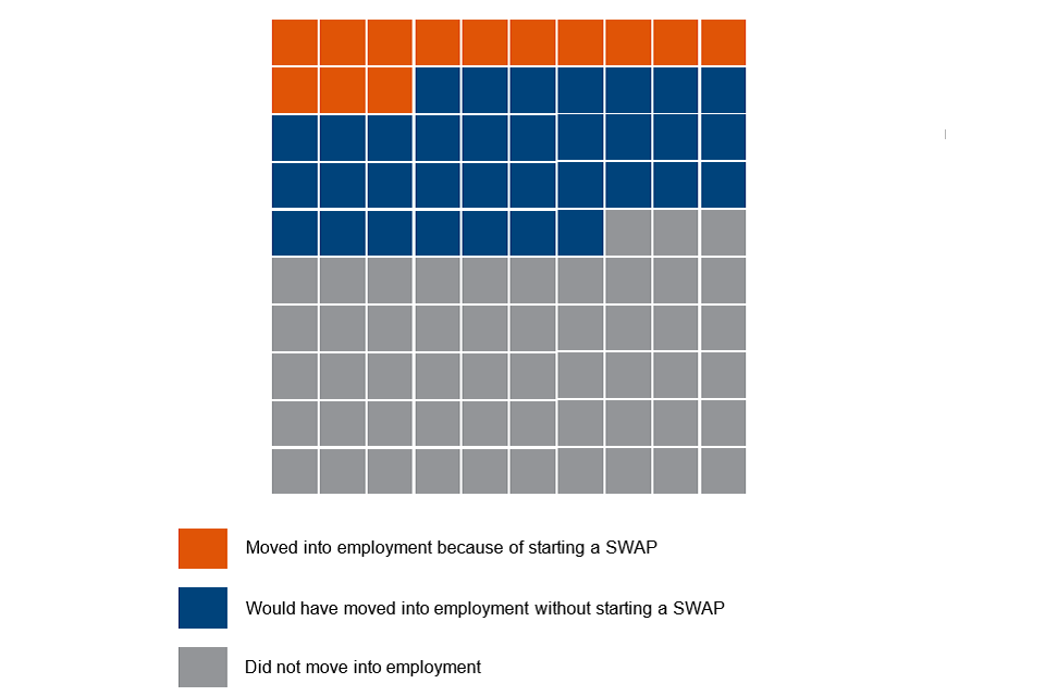
Chart 3.1 shows the net employment impact of participating in a SWAP, 24 months after having started a SWAP. The orange area represents the additional impact that participation in a SWAP has on individuals’ employment outcomes, blue shows the proportion of people who would have moved into employment even without having started a SWAP, and grey shows the proportion who did not move into employment with or without starting a SWAP.

Starting a SWAP has a net impact of 12.5 percentage points (ppts) with a 95% confidence interval (CI) of ±0.4 ppts. This means that for every 100 people that started a SWAP, approximately an extra 13 would be in employment 24 months after their start date compared to 100 people with very similar characteristics who did not start a SWAP. This result is at the average level so while on average 13 more people moved into work because of starting a SWAP, at an individual level, there may be some people who were negatively impacted by starting a SWAP. It is possible that some participants may have been in work in the counterfactual but out of work in the treated scenario. However, we cannot know for certain what would have occurred in the counterfactual.

For every 100 people that started a SWAP, 34 would be in employment 24 months after their start date even if they did not start a SWAP. This is based on the outcomes of the comparison group, where 34% would be in employment based on wider economic conditions. A SWAP is not the only way for customers to find a job, and many were able to find employment through the wider labour market or other employment schemes.

Of the 100 people that started a SWAP, the remaining 53 are not in employment at the 2 year mark or may have been in short employment spells over this time and happened to be out of employment at the 24 month mark. They may also have pursued further training during this time instead of employment.

Chart 3.1 Net employment impact of SWAP 24 months after starting a SWAP

3.4. Longitudinal Impacts on Employment

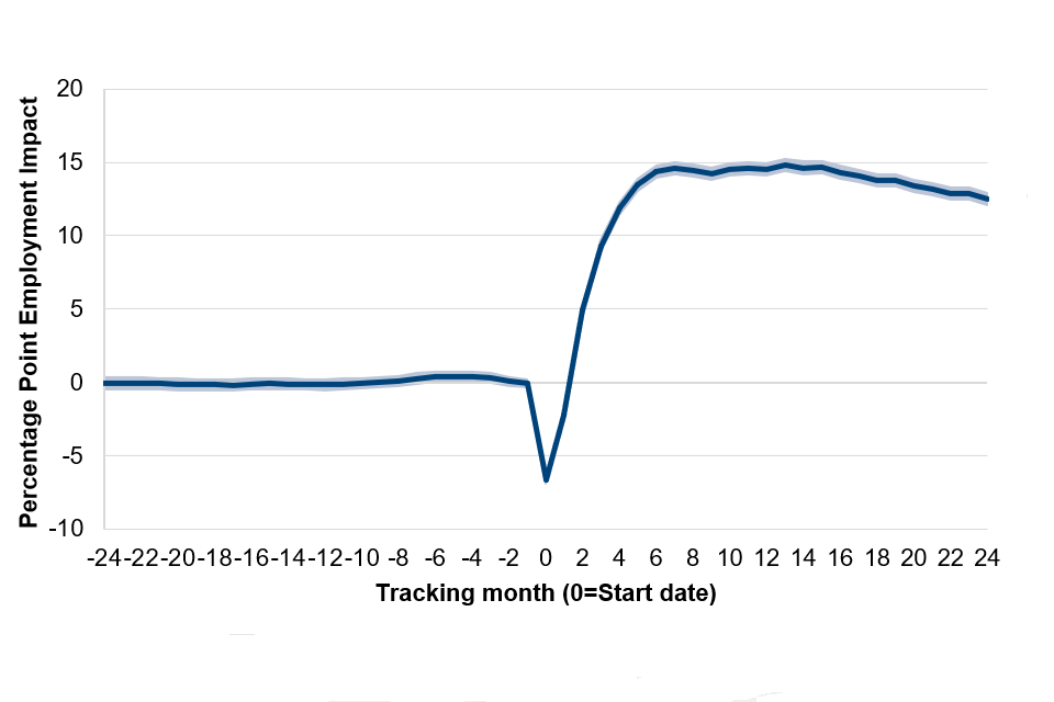
Chart 3.2 shows the longitudinal impact of starting a SWAP on participants’ employment outcomes to assess how the net impact changes over time.

SWAP participants initially experienced a ‘lock-in’ effect in the first month and a half after starting the programme. This reflects the length of a SWAP which, as discussed in section 1, can be up to 6 weeks. During this period, lock-in is likely because participants have less availability for job search activity and so are less likely to find employment during this period (the WEP does not count as time spent in employment). By contrast, while customers in the treatment group are taking part in a SWAP, those in the comparison group continue their job search activity and move into employment. Some customers are also more likely to remain unemployed for longer than they would have done in the absence of the programme in order to complete their participation in the programme.

Following this lock-in, participants were then significantly more likely to be in employment across the remainder of the tracking period.

From month 2 post-SWAP the additional employment impact rises quickly reaching almost 15ppts after 6 months. From month 6, the impact remains roughly stable reaching a peak just below 15ppts in month 13. Beyond month 13 the impact starts to fall, reaching 12.5ppts after 24 months. Translating percentage point impacts to days, participants spent on average 90 days more in employment during the 24 months following a SWAP start than someone who did not start a SWAP^{[footnote 12]}.

As discussed in section 3.2, RTI records are based on calendar months, so if somebody completes a SWAP and moves immediately into employment, it may take an additional month for their earnings to appear in the system depending on when they are paid. Also, not everyone is paid at the same time or the same frequency, so this can create temporary lags on this measure.

Looking at the trajectory of the impact shown in chart 3.2, there is evidence to suggest the impact of starting a SWAP extends beyond the tracking period. Whilst there is a diminishing trend at the end of the tracking period, given the slope we expect any continued fall in the impact to be gradual.

Consistent close agreement of outcomes for treatment and comparison groups before month 0 reflects the success of the matching process as described in section 2. Additionally, the sampling errors shown by the light shaded areas are very small, so the margin of sampling error in these results is very low.

Chart 3.2 Longitudinal employment impact of starting a SWAP

Time in months (0 = start date)	Line PPT
-24	-0.07
-23	-0.07
-22	-0.06
-21	-0.09
-20	-0.12
-19	-0.17
-18	-0.16
-17	-0.18
-16	-0.11
-15	-0.09
-14	-0.13
-13	-0.14
-12	-0.17
-11	-0.12
-10	-0.08
-9	0.02
-8	0.10
-7	0.26
-6	0.37
-5	0.37
-4	0.36
-3	0.30
-2	0.07
-1	-0.06
0	-6.65
1	-2.24
2	4.93
3	9.26
4	11.86
5	13.46
6	14.36
7	14.56
8	14.42
9	14.19
10	14.49
11	14.58
12	14.52
13	14.79
14	14.63
15	14.67
16	14.33
17	14.09
18	13.77
19	13.75
20	13.37
21	13.21
22	12.88
23	12.84
24	12.50

Figures rounded to nearest 2 decimal places

3.5. Sub-Group Analysis

The analysis described in the sections above was repeated for a number of subgroups to understand for which groups participation in a SWAP is most effective.

The subgroups examined were as follows:

• age groups
• regions
• clusters
• demographic characteristics
• time spent receiving benefits pre-start
• quarterly cohorts

The methodology used was identical to that used for the main cohorts, with the addition of a filter applied to both the participant and comparison groups prior to applying PSM so that only the appropriate individuals were retained in both. In all cases the proportion of participants on support following matching was over 99%. All results presented in this section are statistically significant at a confidence level of 95%.

All charts in this section compare sub-groups to the main model results in chart 3.1. The blue section is equivalent to the counterfactual outcome – the proportion of people moving into work irrespective of starting a SWAP. The orange section looks at the net impact of starting a SWAP specifically.

3.5.1. Age Groups

Chart 3.3 looks at the employment impact of starting a SWAP for different age groups. On average, the additional employment impact of starting a SWAP is highest for older participants, especially 50+ year olds. This age group also has the lowest baseline outcome, suggesting that a SWAP is particularly effective here in helping participants who would typically have lower labour market outcomes.

Chart 3.3 Employment impact by age group

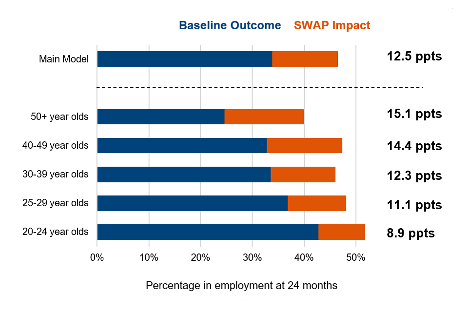
Age group	Baseline Outcome: % in employment at 24 months	SWAP Impact: % in employment at 24 months
Main Model	34%	13%
20 to 24 year olds	43%	9%
25 to 29 year olds	37%	11%
30 to 39 year olds	34%	12%
40 to 49 year olds	33%	14%
50+ year olds	25%	15%

Percentages rounded to nearest whole number

3.5.2. Regions

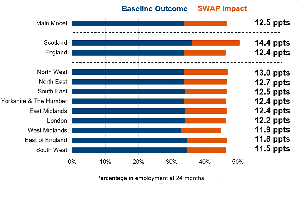
Chart 3.4 looks at the employment impact of starting a SWAP in different regions. The baseline outcome in England is 34%; this baseline outcome is consistent across most regions in England except for the West Midlands where the baseline outcome is lower. There is some small variation across regions but on balance, the additional employment impact of starting a SWAP appears to be similar across England with only a difference of 1.5 ppts across the regions. The highest additional employment impact is in the North West (13.0 ppts) and the lowest is in the South West (11.5 ppts).

The biggest difference in employment impacts is between England and Scotland. The additional employment impact of starting a SWAP in Scotland is higher compared to in England and also the highest impact regionally. The baseline outcome in Scotland is also higher leading to over 50% in employment.

Chart 3.4 Employment impact by region

Region	Baseline Outcome: % in employment at 24 months	SWAP Impact: % in employment at 24 months
Main Model	34%	13%
Scotland	36%	14%
England	34%	12%
North West	34%	13%
North East	34%	13%
South East	34%	12%
Yorkshire and The Humber	34%	12%
East Midlands	34%	12%
London	34%	12%
West Midlands	33%	12%
East of England	35%	12%
South West	35%	11%

Percentages rounded to nearest whole number

3.5.3. Clusters

Chart 3.5 looks at the employment impact of starting a SWAP in different labour market clusters.

Regional analysis masks considerable differences in labour market outcomes at the local labour market level within regions. Focus on regions can also obscure the fact that that there are similarities in local labour markets that are not geographically close to each other.

As outlined in the Analytical Annex of the Get Britain Working White Paper^{[footnote 13]}, the Department has conducted ‘cluster analysis’ to categorise local authorities (LAs) into ‘labour market types’, based on key labour market variables, rather than geographic location.

There are 14 labour market clusters; Chart 3.5 focuses on the employment impact in the 6 clusters with the largest treatment group sample size.

Compared to the regional analysis above, there is slightly more variation in the baseline outcomes and additional SWAP impact across the different clusters. For individuals in LAs in the industrial retirement cluster, both the baseline outcome and the additional SWAP impact are the lowest of the clusters considered. For individuals in LAs in the big cities cluster, while the additional SWAP impact is high at 12.7 ppts, the baseline outcome is one of the lowest of the clusters considered.

Chart 3.5 Employment impact by cluster

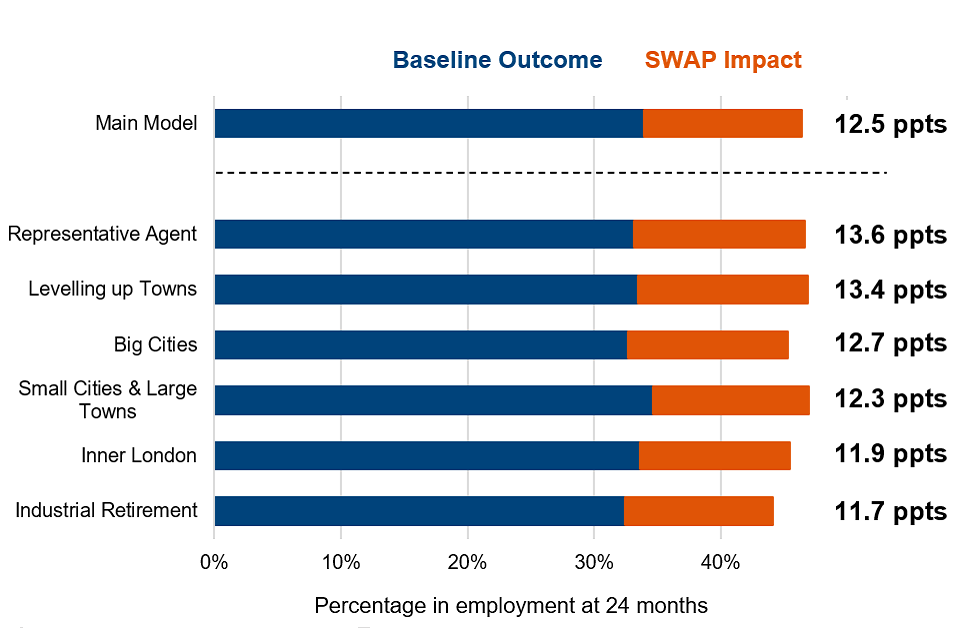
Cluster	Baseline Outcome: % in employment at 24 months	SWAP Impact: % in employment at 24 months
Main Model	34%	13%
Representative Agent	33%	14%
Levelling up Towns	33%	13%
Big Cities	33%	13%
Small Cities and Large Towns	35%	12%
Inner London	34%	12%
Industrial Retirement	32%	12%

Percentages rounded to nearest whole number

3.5.4. Demographic Characteristics

Chart 3.6 looks at the employment impact of starting a SWAP for individuals with different demographic characteristics. Both the additional employment impact and the baseline outcome are higher for female participants with over 50% in employment 2 years after starting a SWAP. The difference in the additional SWAP impact between male and female participants may be linked to the sectors in which they participate. For example, most of the participants who start a SWAP in construction are male and as shown in Appendix C, the additional impact for those who start a construction SWAP is only 5.0 ppts.

For individuals with a current health-related restriction to work, the baseline outcome is 17% which is lower than for those with a historic health-related restriction to work. However, the SWAP impact for those with a current restriction to work is higher at 15 ppts. One caveat here is that the impact for those with a current restriction to work has been found using a very small number of individuals (approximately 1% of the treatment group) so these results may be subject to large sampling error. Despite this caveat, the result is statistically significant at a confidence level of 95%.

Chart 3.6 Employment impact by demographic characteristics

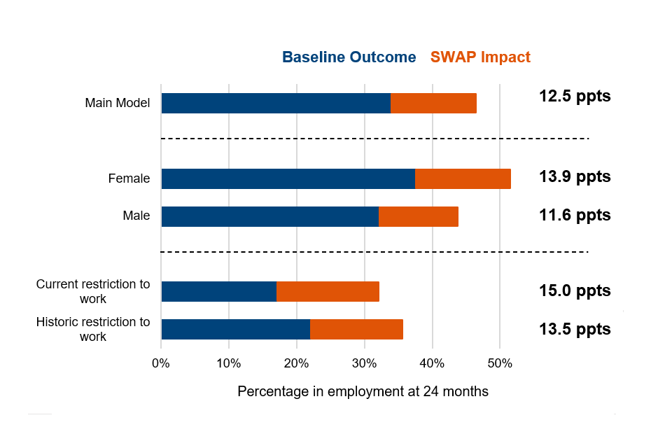
Characteristic	Baseline Outcome: % in employment at 24 months	SWAP Impact: % in employment at 24 months
Main Model	34%	13%
Female	38%	14%
Male	32%	12%
Current restriction to work	17%	15%
Historic restriction to work	22%	14%

Percentages rounded to nearest whole number

3.5.5. Time spent receiving benefits pre-start

Chart 3.7 looks at the employment impact of starting a SWAP depending on how many consecutive months a customer spent receiving benefits before starting.

The additional impact of starting a SWAP is higher the longer someone had been in receipt of benefits prior to a SWAP despite a lower baseline.

The additional employment impact of starting a SWAP is highest for participants who spent more than 1 year in receipt of benefits before starting a SWAP. These participants have the lowest baseline outcome with only 28% in employment. The 13.5 ppts SWAP impact acts as a leveller for these participants bringing the total proportion in employment to over 40%. This result suggests that a SWAP is more effective at helping participants who are further from the labour market.

For participants who spent 7 to 12 months in receipt of benefits, the additional employment impact of starting a SWAP is higher compared to those who spent 4-6 months in receipt of benefits before starting. However, the overall proportion in employment is 52% for both groups as the baseline outcome is higher for the 4-6 months group.

Meanwhile, even though the overall proportion in employment for the 1 to 3 months group is over 55%, this figure is mostly driven by the high baseline outcome of 48%. The actual SWAP impact is only 8.1 ppts^{[footnote 14]}.

Chart 3.7 Employment impact by time receiving benefits pre-start

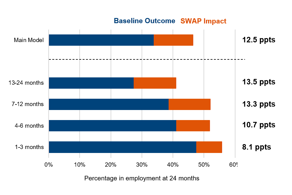
Months	Baseline Outcome: % in employment at 24 months	SWAP Impact: % in employment at 24 months
Main Model	33%	13%
13 to 24 months	27%	13%
7 to 12 months	39%	13%
4 to 6 months	41%	11%
1 to 3 months	48%	8%

Percentages rounded to nearest whole number

3.5.6. Quarterly Cohorts

Chart 3.8 looks at the employment impact of starting a SWAP for the quarterly cohorts within the 2021 to 2022 financial year. The April 2021 to March 2022 cohort used in the main model was split into 4 separate cohorts: April 2021 to June 2021, July 2021 to September 2021, October 2021 to December 2021, and January 2022 to March 2022.

By splitting the year into quarters, we can look at if, and how, the additional employment impact of starting a SWAP varies throughout the year.

There is substantial variation in the additional employment impact for different cohorts in the 2021 to 2022 financial year. The earliest cohorts have better outcomes than later cohorts – a higher proportion of the April 2021 to June 2021 cohort are in employment at 24 months (regardless of whether they started a SWAP) and the additional employment impact of starting a SWAP is also higher for earlier cohorts.

This difference in employment outcomes may be due to external factors. During the COVID-19 pandemic, the group of customers receiving benefits was more diverse. As lockdown restrictions eased in 2021, labour market interventions like SWAP may have been more effective due to more and different vacancies and opportunities in the jobs market.

Given the variation in the additional employment impact between the April 2021 to June 2021 cohorts and the January 2022 to March 2022 cohorts, the lower additional employment impact of 9.6 ppts experienced by the later cohorts is used as a sensitivity check in the cost benefit analysis in section 4.3.

Chart 3.8 Employment impact by quarterly cohort

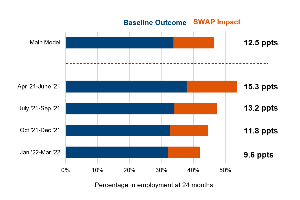
Quarterly cohort	Baseline Outcome: % in employment at 24 months	SWAP Impact: % in employment at 24 months
Main Model	34%	13%
Apr 2021 to June 2021	38%	15%
July 2021 to Sep 2021	34%	13%
Oct 2021 to Dec 2021	33%	12%
Jan 2022 to March 2022	32%	10%

Percentages rounded to nearest whole number

3.6. Sensitivity Analysis

Sensitivity analysis has been conducted to ensure that the analysis is robust when considering different methodologies. As discussed in section 2.3, education and ethnicity variables have not been included as matching characteristic variables in the main model due to coverage limitations. The inclusion of education and ethnicity variables as matching variables has been tested in this section first using LEO and then using LILR.

One potential issue with this section of the analysis is the risk of the multiple comparison problem. By comparing a variety of different characteristics and looking at the trends, there is a risk that different trends could occur not because the impact of starting a SWAP is inconsistent across different groups, but because of smaller sample sizes or sampling errors. This sensitivity analysis is exploratory and corrections for multiple comparisons have not been applied, so caution should be applied when considering the heterogeneity of the results. However, given the relatively large sample size of these groups, and the results also show no significant deviations from the trend results, the multiple comparison problem is unlikely to be an issue.

3.6.1. Including LEO variables

To include variables from the LEO dataset^{[footnote 15]} in the group of characteristics used for matching the treatment and comparison groups, the main model needed to be restricted to only those with a LEO record. As the LEO dataset only has full coverage for individuals educated in England and younger than 40, several restrictions were added to the model to isolate the effect of including LEO variables as matching variables.

As with the main model, data cleaning is also done to remove individuals with missing LEO characteristics data.

Table 3.1 shows the different scenarios that were considered in relation to the main model to compare the effect of including LEO variables as matching variables.

Table 3.1 Adjustments to the Main Model – LEO

Model	Difference
England	Geographical restriction - Individuals located in Scotland were removed
England, 20 to 40	Age restriction - Individuals located in Scotland and older than 40 years old were excluded
England, 20 to 40 w/ a LEO record	LEO record restriction - Only individuals who were located in England, aged between 20 and 40 years old and had a LEO record were included
Including LEO variables for matching	The same restrictions as the previous models were applied and LEO variables were included as matching variables

Chart 3.9 below shows how the employment impact changes as these different restrictions are introduced. The net impact shown on the right-hand side also takes into account the DiD adjustment described in section 2.1.

As the main model is restricted, the employment impact of starting a SWAP falls. This is to be expected given the findings of the subgroup analysis in section 3.5. The geographical restriction limiting the model to those located in England leads to a small 0.1 ppt fall while the age restriction leads to a further 1.4 ppts fall to an impact of 11.0 ppts. When the model is further restricted to only those with a LEO record, the employment impact falls to 8.8 ppts. Finally, when LEO variables are included as matching variables (for the same group of those with a LEO record), the employment impact is 9.0 ppts. This is not statistically different from the employment impact when LEO variables were not included for matching.

While we cannot know what impact including education, ethnicity and other LEO variables would have had on the results for the whole cohort due to the data coverage limitations, when LEO variables are included for the eligible cohort, we can see that not including LEO variables has not negatively biased the results.

Chart 3.9 Employment impact of starting a SWAP – LEO restrictions

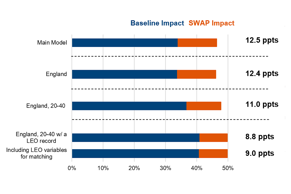
LEO restrictions	Baseline Outcome %	SWAP Impact %
Main Model	34%	13%
England only	34%	12%
England only, 20 to 40 years old	37%	19%
England, 20 to 40 w/ a LEO record	41%	9%
Including LEO variables for matching	41%	9%

Percentages rounded to nearest whole number

3.6.2. Including LILR variables

As discussed in Section 2.3, data from the LILR is included within the LEO dataset, only covers post-16 education and like LEO, does not have full coverage outside of England. However, unlike LEO, the LILR covers all age groups which means LILR can be used to provide ethnicity data and some education data coverage.

To include variables from the LILR dataset^{[footnote 16]} in the group of characteristics used for matching the treatment and comparison groups, the main model needed to be restricted to only those with a LILR record. As in the previous section, a few restrictions were added to the model to isolate the effect of including LILR variables as matching variables.

As with the main model, data cleaning is also done to remove individuals with missing LILR characteristics data.

Table 3.2 shows the different scenarios that were considered in relation to the main model to compare the effect of including LILR variables as matching variables.

Table 3.2 Adjustments to the Main Model – LILR

Model	Difference
England	Geographical restriction - Individuals located in Scotland were removed
England, w/ a LILR record	LILR record restriction - Only individuals who were located in England and had a LILR record were included
Including LILR variables for matching	The same restrictions as the previous models were applied and LILR variables were included as matching variables

Chart 3.10 below shows how the employment impact changes as these different restrictions are introduced. The net impact shown on the right-hand side also takes into account the DiD adjustment described in section 2.1.

As with the LEO restrictions in the previous section, as the main model is restricted, the employment impact of starting a SWAP falls. When the model is further restricted to only those with a LILR record, the employment impact falls to 10.8 ppts. Restricting the model to only include individuals with a LILR record introduces a source of bias. The training element of a SWAP in England is likely to be recorded in the LILR. This means that individuals in the treatment group may be more likely to have a record in the LILR. By contrast, while individuals in the comparison group may have qualifications, these qualifications will not necessarily have been recorded in the LILR. This means they will not be included when the model is restricted to only those with a LILR record; this could explain the lower impact seen.

When LILR variables are included as matching variables (for the same group of those with a LILR record), the employment impact is 10.7 ppts. This is not statistically different from the employment impact when LILR variables were not included for matching.

Given the limitations of the LILR dataset, we cannot truly know whether education history and ethnicity has been fully controlled for. Nor do we know what impact including education and ethnicity variables from the LILR would have had on the results for the whole cohort due to the data coverage limitations. However, similarly to the findings in the previous section, when LILR variables are included for the eligible cohort, we can see that not including LILR variables has not negatively biased the results.

Chart 3.10 Employment impact of starting a SWAP – LILR restrictions

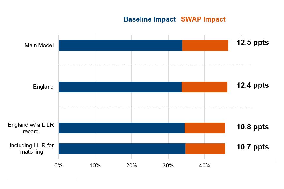
LILR restrictions	Baseline Outcome %	SWAP Impact %
Main Model	34%	13%
England only	34%	12%
England w/ a LILR record	35%	11%
Including LILR for matching	35%	11%

Percentages rounded to nearest whole number

3.7. Discussion of Results

The analysis shows that SWAP was successful in supporting participants into employment. At 2 years after start, for every 100 people who started a SWAP, an additional 13 individuals moved into unsubsidised employment, compared to 100 similar individuals who did not participate. These results remain high over time, with the impact increasing quickly in the first 6 months after starting a SWAP, reaching a plateau which holds up to month 13, and then gradually falling. Despite the falling impact towards the end of the tracking period, the trend appears to show a slow decline. This provides some confidence the positive impacts of the scheme persist into the future, even if the impact does not remain as high.

In most regions considered, except for Scotland, both the proportion of people moving into work and the additional SWAP impact are very similar. However, when other subgroups are considered such as age groups and different demographics, the results show that starting a SWAP tended to have a higher impact for the more disadvantaged groups who have lower baseline employment outcomes. This finding could have implications for future SWAP policy design.

As discussed in Section 1, the sector-based work academies that ran from 2011 to 2020 were previously evaluated in 2016. While the cohorts considered in the 2016 evaluation differ from the cohorts used in this analysis, the programme design has remained similar. The 2016 evaluation looked at the impact of sector-based work academies on 2 cohorts of 19 to 24 year old JSA claimants who started in 2011 to 2012 and 2012 to 2013 respectively. The report estimated that the additional employment impact for the 2011 to 2012 cohort was 9 ppts at 104 weeks (2 years) after starting a SWAP and for the 2012 to 2013 cohort was 9 ppts at 78 weeks (eighteen months) after starting a SWAP. Though this is lower than the additional employment impact estimated for the main model in this evaluation, this is similar to the subgroup analysis findings on age (described in Section 3.5.1) which showed that the additional employment impact of starting a SWAP for 20 to 24 year olds is 8.9 ppts.

4. Cost Benefit Analysis

This section presents a cost benefit analysis (CBA) of the Sector-based Work Academy Programme (SWAP) for the 2021 to 2022 cohort of SWAP participants in receipt of Universal Credit (UC). The CBA considers the costs and benefits of SWAP within 24 months of participants starting the programme. While the impact estimated in the previous section was found using a sample of SWAP participants, the results in this section apply to everyone in receipt of UC who started a SWAP.

The methodology used for this CBA is outlined in section 4.1; the baseline findings are presented in section 4.2; and findings from sensitivity checks are presented in section 4.3.

4.1. Methodology

The methodology underpinning the CBA of SWAP is based on guidance from the Green Book^{[footnote 17]} and uses the Department for Work and Pensions Social Cost Benefit Analysis (SCBA) model. This approach is consistent with previous departmental impact assessments (Cann, 2024). The CBA is based on the impacts set out in section 3; for the SCBA model, these impacts are converted into additional days in unsubsidised employment. Over the 24-month period following a SWAP start, an individual spent on average an additional 90 days in unsubsidised employment compared to those who did not start a SWAP.

The application of this approach is outlined below in terms of:

• whose perspective is considered – section 4.1.1
• which costs and benefits are estimated – section 4.1.2
• the limitations of this methodology – section 4.1.3

4.1.1. The perspectives under consideration

The costs and benefits of SWAP are considered from 4 key perspectives:

• the SWAP participants (henceforth referred to as ‘the participants’)
• the participants’ employers
• the Exchequer (the Government budget perspective)
• society

The participant perspective focuses on individual costs and benefits, such as changes in wages, benefits, and taxes as a result of additional time in unsubsidised employment.

The employer perspective considers the cost to employers of paying participants and the benefits from the additional output produced by participants.

The Exchequer perspective refers to the fiscal costs and benefits of the programme, including changes in tax revenue and benefit expenditure, as well as the cost of funding the sector-based work academy programme.

The society perspective represents an aggregate of all British citizens. This means that a cost or benefit to participants, their employers or the Exchequer can also represent a cost or benefit to society. Many of the gross impacts are essentially “transfer payments”. Transfer payments represent a cost to one group of citizens but a benefit to another. For example, the wages earned during additional employment as a result of going on a SWAP represent a benefit to participants but a cost to their employers. Transfer payments therefore cancel out when estimating the net benefits or costs of a policy from society’s perspective. The programme leads to a net benefit to society through the increase in output that occurs when participants who were previously unemployed and producing no output, produce output during the additional time spent in unsubsidised employment as a result of the programme. This additional output represents a net benefit to employers and society.

For this report, all perspectives will be measured for the baseline estimates while the sensitivity analysis will focus on the perspectives of the Exchequer and society.

4.1.2. The costs and benefits under consideration

Table 4.1 summarises the impacts of SWAP which have been translated into monetised costs and benefits for this CBA. These impacts and the associated costs and benefits are discussed in more detail below.

Once the costs and benefits have been estimated, a Cost Benefit Ratio (CBR) is produced which reflects the balance of the 2. If the ratio is greater than £1, then for every pound spent on the SWAP, more than one pound is generated in return.

Table 4.1 Monetised costs and benefits of the Sector-based Work Academy Programme

Perspective

SWAP programme impact (24 months)	Participants	Employer	Exchequer	Society
Increase in output	0	+	0	+
Increase in wages post SWAP	+	–	0	0
Programme costs	0	0	–	–
Reduction in operational costs	0	0	+	+
Reduction in benefits post SWAP	–	0	+	0
Increase in taxes	–	–	+	0
Increases in travel & childcare costs post SWAP	–	0	0	–
Redistributive costs and benefits	+	0	0	+
Social cost (benefit) of Exchequer finance	0	0	0	0

Key: ‘+’ denotes a net benefit; ‘–’ denotes a net cost; ‘0’ denotes neither cost nor a benefit.

Increase in output

This refers to the economic output produced by participants as a result of additional time spent in unsubsidised employment. This output represents a benefit to employers (who sell it) and society (who consume it). The Department for Work and Pensions (DWP) does not have information on the value of this output, so it is necessary to make a number of simplifying assumptions.

The labour market is assumed to be perfectly competitive. This implies that employers will hire workers up to the point where the value of an additional unit of output is equal to the associated marginal cost of production. The cost of production, and therefore the value of the output produced during additional spells in unsubsidised employment, is assumed to be equal to the commensurate gross wage payments and employers’ National Insurance (NI) contributions.

Increase in wages post SWAP

This refers to the gross wages received by participants during additional time spent in employment after the programme. Wages represent a benefit to participants but a cost to their employers. This means they do not represent a net cost or benefit to society as a whole, except via redistributive effects described below.

Programme costs

For the baseline CBA estimates, the cost per SWAP has been estimated to be £428. This cost has been estimated using reported figures from DWP and DfE financial records from 2021 to 2022.

The £428 cost per SWAP includes

• administration costs of £101 (funded and recorded by DWP)
• the cost of the PET element of £327 (funded and recorded by DfE in England)

The DWP costs cover the staff and non-staff costs associated with brokerage time for employment advisors, referral interview time for jobcentre staff, and average FSF payments to support travel and childcare costs during participation in the programme.

Not every SWAP requires DfE funding for the PET element; the training element for some of the programmes may be funded by employers or charities, or in some cases the training is funded through the FSF. Therefore, the £327 cost of the PET element has been calculated using the total amount of AEB spend as recorded by DfE (approximately £22 million) and dividing this by the total number of SWAP starts in England (approximately 67,000). For the CBA, it is assumed that the unit cost of a SWAP was the same in Scotland.

These estimates are lower than the cost per SWAP assumed in the 2020 Spending Review which was approximately £752. This was made up of £222 of DWP funding and £530 of DfE funding per SWAP.

This difference in DWP costs may be due to difficulties in recording precise SWAP-associated staff and non-staff costs for employer advisors and JCP staff, for example, if the time spent setting up and administering a SWAP only represents a fraction of how their total time is divided. It could also mean the scheme was administered more efficiently than assumed at its inception.

While we know that not all SWAP participants undertake AEB funded learning, only around 18,000 SWAP participants were reported as having undertaken training funded through the AEB in the 2021 to 2022 financial year. This represents just over a quarter of the total SWAP starts in England and the average training cost for these participants was around £1200 per start^{[footnote 18]}. The calculation of the unit cost of £327 assumes that only SWAP training that is explicitly recorded as such on the ILR is funded by DfE.

With only a quarter of SWAP starts recorded on the ILR as being AEB funded, it is likely that there is underreporting on the ILR of AEB funded SWAP training. In some cases, though training is recorded for participants, it is not always flagged as part of the SWAP. If it is the case that this training is indeed a participant’s SWAP training element, then there may be a large amount of DfE spend on these SWAP participants which we have not been able to account for. The DfE assumption of £530 per SWAP assumes that there are a greater number of programmes with AEB funded training elements across England, while still assuming that not all training is AEB funded.

Given the uncertainty around the cost of a SWAP, sensitivity analysis is conducted in section 4.3 using the higher unit cost of £752, which may be a more representative cost if there is underreporting of SWAP spend on the ILR. These payments represent a cost to the Exchequer and society, as this diverts economic resources from alternative uses, but no cost to participants or employers as they do not pay directly for SWAP programme costs.

Reduction in operational costs

As shown in Section 3, SWAP has a positive employment effect on participants. This will reduce operational costs as participants will need less support from JCP advisers. As a result, this also means participants are less likely to participate in other DWP employment programmes. This translates into operational savings which represent a benefit to the Exchequer and society, as economic resources can be reallocated to alternative uses.

Reduction in benefits post SWAP

This refers to the net reduction in benefit entitlement and take up that occurs when participants spend additional time in employment as a result of participation in a SWAP. This represents a cost to participants but a benefit to the Exchequer. This means there is no net cost or benefit to society, except via redistributive effects as explained below. Changes in benefit entitlement and take up are estimated using the DWP Policy Simulation Model^{[footnote 19]}.

Increase in taxes

This refers to the increase in income tax, National Insurance and indirect tax revenue that occurs when participants spend additional time in unsubsidised employment as a result of participation in a SWAP. This represents a benefit to the Exchequer but a cost to both employer and participants. Therefore, there is no net cost or benefit to society, except via redistributive effects as discussed below.

Increases in tax revenue are estimated using the DWP Policy Simulation Model^{[footnote 20]}. The costs and benefits associated with the remaining sector-based work academy impacts are described briefly below. For a detailed description of the methodologies used to estimate these costs and benefits, see Fujiwara (2010).

Increase in travel and childcare costs

This refers to the additional travel and childcare costs that are incurred by participants during additional employment as a result of participation in a SWAP. This also represents a cost to society as the provision of additional travel and childcare services diverts economic resources from alternative uses.

Redistributive costs and benefits

This refers to the redistributive costs and benefits associated with monetary transfers between participants, employers and the Exchequer. In line with the methodology prescribed in the HM Treasury Green Book, participants, who have relatively low incomes, are assumed to value each additional pound more highly than employers and the average taxpayer, both of whom have a relatively high income compared to participants. This implies, for example, that monetary transfers from the Exchequer to participants represent a benefit to society. In line with the recommendations of Fujiwara (2010), redistributive costs and benefits are estimated by applying a ‘welfare weight’ of 2.4 to monetary transfers made to and from programme participants.

Social Cost (or benefit) of Exchequer Finance (SCoEF)

This refers to the cost of raising the tax revenue that was required to finance SWAP. This ‘deadweight loss’ arises because taxation creates market distortions which have an adverse effect on economic efficiency. The distribution of the social cost of Exchequer finance amongst members of society depends on the specific details of taxation policy. For the purposes of this analysis, it is assumed to accrue to society as a whole. In line with the recommendations of Fujiwara (2010), the social cost of Exchequer finance is assumed to equate to 20% of the net cost of the programme to the Exchequer. However, as this estimate is subject to considerable uncertainty, it is only considered as part of sensitivity analysis (see section 4.3).

4.1.3. Limitations of this approach

The CBA estimates presented in section 4.2 are subject to 2 main caveats. First, the accuracy of the estimates depends on the robustness of the impact estimates from which they are derived (see section 3) and the validity of the assumptions upon which they are based (see section 4.1.2). Uncertainty regarding these inputs has been partially mitigated by undertaking sensitivity analysis (see section 4.3).

Second, the CBA estimates exclude a number of potentially significant costs and benefits due to a lack of robust evidence^{[footnote 21]}. For example, it has not been possible to obtain robust estimates relating to:

• the additional leisure time which participants forego (this represents a potential cost to participants and therefore society)
• the non-pecuniary benefits associated with additional time in unsubsidised employment (these represent a potential benefit to participants and therefore society)
• the cost of the training element of the SWAP when not funded through the AEB (this represents a potential cost to employers or the Exchequer in some places and therefore society)
• the cost of the WEP and GJI (this represents a potential cost to employers and therefore society)
• any additional output produced by participants during the WEP (this represents a potential benefit to employers and therefore society)
• the cost of hiring and training incurred by employers (this represents a potential cost to employers and therefore society)
• the reduction in crime^{[footnote 22]} which may result from the programme (this represents a potential benefit to society)
• the economic multiplier effect which may result from the programme (this represents a potential benefit to society)

These non-monetised costs and benefits should be borne in mind when interpreting the CBA estimates presented in section 4.2.

4.2. Results of cost benefit analysis

Table 4.2 below presents estimates of the costs and benefits of the SWAP at 24 months post-programme which are based on the following baseline assumptions:

• the value of the output produced during additional unsubsidised employment is equal to the commensurate gross wage payments and employers’ NI contributions; and
• the SWAP results in redistributive costs and benefits but does not result in substitution effects or a social cost (or benefit) of Exchequer finance.

The estimates presented in this section are expressed in 2021 to 2022 prices and have been discounted to account for social time preference^{[footnote 23]}.

Table 4.2 Estimated Costs and Benefits of the Sector-based Work Academy Programme for UC customers under baseline assumptions

Perspective

SWAP programme impact (24 months)	Participants	Employer	Exchequer	Society
Increase in output	0	+1,520	0	+1,520
Increase in wages post SWAP	+1,450	-1,450	0	0
Programme costs	0	0	-430	-430
Reduction in operational costs	0	0	+20	+20
Reduction in benefits post SWAP	-440	0	+440	0
Increase in taxes	- 250	-70	+320	0
Increase in travel and childcare costs	-30	0	0	-40
Redistributive costs and benefits	+1,080	0	0	+1,080
Social cost (benefit) of Exchequer finance	0	0	0	0
Total Benefits	+2,530	+1,520	+780	+2,620
Total Costs	-720	-1,520	-430	-460
Net Benefit	+1,810	0	+360	+2,160
Cost Benefit Ratio (CBR)	3.50	1.00	1.83	5.66

Note: The figures in the table have been rounded to the nearest 10. Components may not sum to total due to rounding.

Participants

Table 4.2 shows that under the baseline assumptions, a SWAP is estimated to result in a net benefit to participants. This is because the additional wages received by participants are expected to outweigh the costs associated with a net reduction in benefit receipt and net increases in tax liabilities, travel and childcare costs. Table 4.2 suggests that, on average, participants are financially better off by approximately £730 as a result of participation in the programme. The assumption that participants value additional income more highly than the average taxpayer means that the programme is also estimated to result in a net redistributive benefit of £1,080, bringing the total net benefit to £1,810. This is equivalent to a CBR of £3.50 per pound spent.

Participants’ Employers

Table 4.2 shows that under the baseline assumptions, a sector-based work academy is estimated to be cost neutral to employers, so the CBR for employers is £1. This is because the value of the output produced is assumed to be equal to the sum of the gross wage payments and employers’ NI contributions. However, it may be the case that the output gained from an employer’s perspective is greater than the wages paid. As discussed in section 4.1.3, this analysis excludes the costs of hiring and training participants so the true costs may be higher.

The Exchequer

Table 4.2 shows that under the baseline assumptions, a SWAP is estimated to result in a net benefit to the Exchequer of approximately £360 per participant. This is because the programme costs are expected to be less than the benefits associated with a net increase in tax revenues and net reductions in benefit expenditure, and operational costs. As Table 4.2 shows, the CBR for the Exchequer is £1.83. This means that for every £1 spent by the Exchequer on a SWAP, after 2 years, the Exchequer gets a return of an additional 83p.

Society

Table 4.2 shows that under the baseline assumptions, a SWAP is estimated to result in a net benefit to society of approximately £1,070 per participant. This is largely due to the additional economic output that is produced by participants during additional spells in unsubsidised employment as a result of participation in a SWAP. The assumption that participants value additional income more highly than the average taxpayer means that the programme is also estimated to result in a net redistributive benefit of £1,080, bringing the total net benefit to society to £2,160. As shown in Table 4.2, the CBR for society is £5.66 and this is the highest CBR across the 4 perspectives. As discussed in section 4.1.3, there are several costs and benefits that are not included in the model due to a lack of robust evidence. However, provided that the costs that were not included sum to less than £2,160 per participant, the SWAP would still result in a net benefit to society.

4.3. Sensitivity Analysis

As discussed in section 4.1, there are a number of assumptions underpinning the CBA model and there is considerable uncertainty regarding the accuracy of these baseline assumptions. Therefore, several sensitivity checks have been used to test these assumptions. These sensitivity checks are summarised in Table 4.3 below and Charts 4.1 and 4.2 below show the results of these sensitivity scenarios on the CBR for the Exchequer and society perspectives at the 2-year mark.

Table 4.3 Summary of baseline assumptions and sensitivity adjustments

Baseline assumptions	Sensitivity check
Redistributive costs and benefits included	Redistributive costs and benefits excluded
No substitution effects	Partial substitution effects of 20% included
Social cost (or benefit) of Exchequer finance excluded	Social cost (or benefit) of Exchequer finance included
Unit cost of £428	Higher unit cost of £752
Additional employment impact of 12.5ppts	Lower additional employment impact of 9.6 ppts at 24 months

Redistributive costs and benefits excluded

The baseline results assume that distributional impacts are present. As discussed in section 4.1.2, participants who have relatively low incomes are assumed to value each additional pound more highly than employers and the average taxpayer, both of whom have a relatively high income compared to participants. As a sensitivity check, this assumption is excluded, and it is assumed that SWAP did not result in redistributive costs or benefits. Under this scenario, the CBR for the Exchequer is unaffected, as shown in Chart 4.1. This is because this assumption is not relevant for the Exchequer calculation, as discussed in section 4.1.2.

Chart 4.2 shows that while the CBR for society remains above the breakeven point, excluding the redistributive costs and benefits leads to a fall in the CBR from £5.66 to £3.32.

Substitution effects included

The baseline model does not assume any substitution effects. As a sensitivity check, it is assumed that the SWAP results in substitution effects of 20%. This assumes that a proportion of the positive employment impacts experienced by participants are obtained at the expense of non-participants. Arguably, due to the nature of sector-based work academies there should be no job displacement caused^{[footnote 24]}.

As chart 4.1 shows, including substitution effects reduces the CBR for the Exchequer from £1.83 to £1.47. This is because the net benefit to the Exchequer falls as the ‘substituted’ non-participants would be expected to pay less tax and receive more benefits than under the baseline assumptions. However, given the relatively low cost per SWAP, the CBR for the Exchequer remains above the breakeven point.

Chart 4.2 shows that including substitution effects also reduces the CBR for society from £5.66 to £4.60. This is mainly because the ‘substituted’ non-participants would be expected to produce less output than under the baseline assumptions which reduces the net benefit to society while the costs remain low. The estimated CBR for society also remains above the breakeven point.

Social cost (or benefit) of Exchequer finance included

The baseline model does not include the social cost (or benefit) of Exchequer finance due to the uncertainty associated with this estimate (as discussed in section 4.1.2).

As a sensitivity check, it is assumed that the SWAP results in a social benefit of Exchequer finance, as the programme results in exchequer savings and so reduces the tax burden.

Chart 4.1 shows that including the social benefit of Exchequer finance has no effect on the CBR for the Exchequer. Meanwhile, Chart 4.2 shows a small increase in the CBR for society from £5.66 to £5.83.

Higher unit cost

As discussed in section 4.1.2, there is some uncertainty surrounding the true cost of the sector-based work academy programme. As a sensitivity check, it is assumed that the cost per SWAP is higher at £752 per SWAP. This was calculated based on estimated costs in the 2021 Spending Review bid and represents the cost ‘ceiling’ for a SWAP.

Chart 4.1 shows that there is a large fall in the CBR for the Exchequer from £1.83 to £1.04. Crucially however, the CBR remains above the breakeven point so even at a higher cost, 2 years on SWAP continues to generate a positive return for the Exchequer.

Chart 4.2 shows that there is also a fall in the CBR for society from £5.66 to £3.33. The CBR change is roughly proportional to the change in the unit cost, as the programme cost makes up the majority of the costs for the analysis. While this sensitivity check leads to the lowest CBR for society, the CBR remains well above the breakeven point.

Lower additional employment impact

The final sensitivity check assumes that the additional employment impact at 24 months post intervention is lower and therefore participants spend fewer days in unsubsidised employment because of a SWAP. As discussed in the subgroup analysis in section 3.5, for later months in the 2021 to 2022 financial year (January 2022 – March 2022), the additional employment impact at 24 months is 9.6 percentage points. This sensitivity check considers the possibility that the higher additional employment impact experienced by earlier cohorts was an anomaly and that this lower additional employment impact experienced by later cohorts is the true additional employment impact.

Chart 4.1 shows that this sensitivity check leads to a fall in the CBR for the Exchequer from £1.83 to £1.35. So, the CBR remains above the breakeven point and the SWAP continues to generate a positive return for the Exchequer.

Similarly, Chart 4.2 shows that if the additional employment impact at 24 months is lower and participants spend fewer days in unsubsidised employment, the CBR for society falls from £5.66 to £4.26.

Chart 4.1 Sensitivity analysis of the Exchequer Cost Benefit Ratio at 2 years

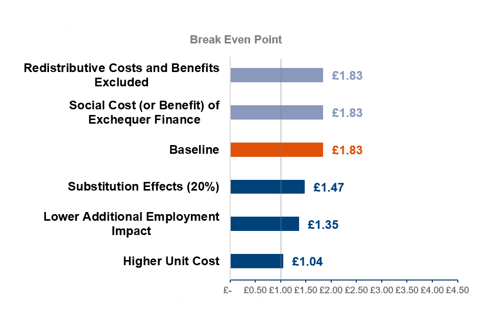
Effect	CBR £
Break even point	£1.00
Redistributive Costs and BenefitsExcluded	£1.83
Social Cost (or Benefit) ofExchequer Finance	£1.83
Baseline	£1.83
Substitution Effects (20%)	£1.47
Lower Additional EmploymentImpact	£1.35
Higher Unit Cost	£1.04

Chart 4.2 Sensitivity analysis of the Society Cost Benefit Ratio at 2 years 

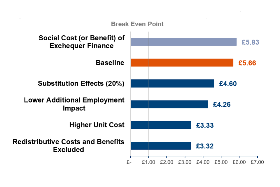
Effect	CBR £
Break even point	£1.00
Social Cost (or Benefit) ofExchequer Finance	£5.83
Baseline	£5.66
Substitution Effects (20%)	£4.60
Lower Additional EmploymentImpact	£4.26
Higher Unit Cost	£3.33
Redistributive Costs and BenefitsExcluded	£3.32

5. Conclusion

5.1. Impact Analysis

The analysis uses a PSM approach to compare employment outcomes between individuals who started a SWAP and UC customers who were eligible for the programme but did not start a SWAP. This methodology allows us to compare similar groups of people directly against each other. The analysis uses a wide variety of characteristic variables to control for different demographic traits that could influence labour market outcomes outside of a SWAP. The aim of this analysis is to assess the direct impact of starting a SWAP, however, as discussed there are limitations of this methodology, and it is impossible to be absolutely confident that we have fully controlled for selection bias.

The results show that starting a SWAP had a positive impact on the likelihood of being in employment. For every 100 people that started a SWAP, approximately an extra 13 would be in employment 2 years after their start date compared to 100 people who did not start who had very similar characteristics.

In terms of additional days in employment, 2 years after starting a SWAP, participants had on average spent 90 days more in employment than someone who did not start a SWAP.

The longitudinal results show that the employment outcomes rise quickly up to month 6 and are then fairly consistent up to month thirteen. There does appear to be a diminishing trend beyond month 13, however the additional employment impact is falling gradually so we can expect the impact of starting a SWAP to extend beyond the 2-year tracking period.

The subgroup analysis shows that while the magnitude of the impact may differ, the positive impact of starting a SWAP holds across different groups. For groups with low baseline employment outcomes that are less likely to move into work, the additional employment impact of starting a SWAP is high suggesting that the programme may be particularly effective at helping groups further from the labour market move into employment.

The cohort subgroup analysis shows that within the financial year considered, the programme has a positive impact across all of the quarterly cohorts and continues to be effective upon reaching its ‘steady state’.

Sensitivity checks were also performed to check the validity of the results and address some of the limitations of the approach. The inclusion of education and ethnicity variables using both LEO and LILR data shows that for the groups which are covered by the LEO and LILR data, excluding these variables from the matching characteristics does not appear to have biased the results.

When compared to the results of the 2016 evaluation of sector-based work academies, the additional employment impact found in this report is higher. However, the groups considered in the 2 evaluations differ as the 2016 evaluation only looked at 19 to 24 year old JSA claimants. The subgroup analysis in this report shows that the additional impact of starting a SWAP for 20 to 24 year olds is similar to the result found in the 2016 evaluation.

5.2. Cost Benefit Analysis

Using the estimated impacts, a CBA was conducted to estimate the cost effectiveness of the programme at 2 years post-participation. Given the high additional employment impact and the relatively low cost of the programme a positive CBR is expected; and the results show that under the baseline assumptions, at the 2-year mark for every pound invested:

• participants benefit by £3.50
• the scheme is cost neutral for employers (the return for employers is £1.00)
• the Exchequer benefits by £1.83, with a sensitivity range of £1.04 – £1.83
• society benefits by £5.66, with a sensitivity range of £3.32 – £5.83

It is important to reiterate that the cost and benefit estimates presented in this paper are subject to the caveats discussed in section 4.1.3. The accuracy of these estimates is dependent on the robustness of the impact estimates from which they are derived and the validity of the assumptions upon which they are based. It should also be borne in mind that a number of potentially significant costs and benefits have been excluded from this analysis due to a lack of robust evidence. These include the non-pecuniary benefits associated with SWAP participation (e.g., improvements in participants’ confidence) and any additional training costs incurred by employers. However, it is notable that under all of the scenarios considered in this analysis, the programme is estimated to result in a net gain to the participants, the Exchequer and society as a whole.

Appendix A: Propensity Score Matching

A.1. Why use propensity score matching?

Propensity score matching is often employed in evaluations of this type in order to more accurately estimate the counterfactual i.e., the outcomes that would have occurred in the absence of a SWAP. It is impossible to measure the counterfactual directly, since we cannot know what outcomes SWAP participants would have attained without intervention, so it is necessary to estimate this figure using outcomes for individuals who did not participate.

Participation in a SWAP is voluntary; it is likely that the group who do not participate will be on average different from those who do as participation may be influenced by personal factors. These personal factors could affect overall outcomes; differences that affect outcomes are known as relevant differences. These personal factors may be observable characteristics such as age or gender, or factors that are not easy to measure (unobservable characteristics) such as motivation or enthusiasm.

For example, the group who volunteer for a SWAP may be on average more motivated and willing to work than those who do not. This is a relevant difference as it is likely to affect this group’s probability of finding work in the subsequent year even without completing a placement.

Any relevant differences between the participant and non-participant groups would introduce bias into the impact estimate if this were calculated using the non-participant group as a whole to estimate the counterfactual. The aim of employing propensity score matching is to eliminate this potential source of bias by creating a comparison group which is identical to the participant group in terms of all relevant characteristics. By matching the 2 groups using a rich dataset of observable characteristics, we attempt as much as possible to control for unobservable characteristics too.

The assumption that the matching has successfully controlled for all factors affecting both the likelihood of participation in the programme and the likelihood of attaining the outcomes under evaluation is referred to as the ‘conditional independence assumption’. If this assumption is met, then the 2 groups being compared should be indistinguishable from 2 groups selected at random from the same population.

In other words, it is assumed that, if the participants did not take part in the intervention, they would have the same outcomes as the comparison group. Therefore, the outcomes of the comparison group can be used as an estimate of what would have happened to the treatment group if they were not treated.

A.2. How propensity score matching is carried out

Diagram A.1 below shows the PSM process. The first step for PSM is to define an overall sample containing both participants and non-participants in the intervention under consideration. The methodology applied to select the samples used in this evaluation is described in Section 2.2.

Once the sample has been defined, PSM is carried out as follows:

1. Data on the characteristics of individuals in the sample are used as the input to a logistic regression model, using a logit approach, to estimate the probability of each individual participating in the scheme. This probability is also known as an individual’s ‘propensity score’.

2. The propensity scores are then used to match participants to individuals in the comparison group with a similar likelihood of participating in the intervention. A nearest neighbour matching approach was used where one participant could be matched to 100 nearest neighbours in the comparison group within a propensity score bandwidth of 0.01.

At the end of this process, the desired outcome is for the majority of participant records to be matched with a record in the non-participant group. The records where matching has been successful are described as ‘on support’. The proportion of records which are on support is one of the main criteria used to assess the quality of the matching result. The degree of common support achieved in this analysis is described in Section 3.1. The other major success factor is the bias reduction achieved by the matching, i.e., how similar the matched comparison group is to the participant group compared with the unmatched comparison group based on their observed characteristics.

By assigning reliable propensity scores, and then assessing people with similar scores across the treatment and comparison group, the groups should have similar characteristics overall, in terms of how likely they are to be treated. Under the conditional independence assumption, this means the only remaining difference between the 2 groups is the treatment effect itself. This methodology allows us to compare similar people across different groups and isolate the treatment effect to calculate it.

Diagram A.1 PSM Process

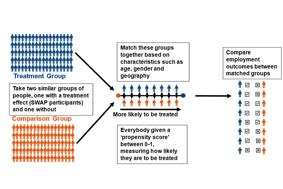
1. Take 2 similar groups of people, one with a treatment effect (SWAP participants) and one without: Treatment Group and Comparison Group

2. Match these groups together based on characteristics such as age, gender and geography. More likely to be treated. Everybody given a ‘propensity score’ between 0 or 1, measuring how likely they are to be treated

3. Compare employment outcomes between matched groups

A.3. Variables used in propensity score matching

The success of PSM depends on the quality and coverage of the data used in the matching and in particular, its ability to control for any factors which affect both selection onto the programme (i.e., if someone participates in SWAP) and the subsequent outcomes of interest (movement into employment).

PSM is considered to be a viable approach for evaluating DWP’s labour market programmes because DWP holds a wide range of data on individuals on its benefit caseload which can be used as the basis of the matching. This includes detailed information on claimants’ benefit and employment histories, which have been shown to be a valid proxy for unobserved but relevant characteristics such as personality traits and motivation (Caliendo, Mahlstedt and Mitnik, 2014).

Table A.1 below lists the variables used as the basis for propensity score matching in this evaluation. The sensitivity analysis explored in Section 3.6 includes variables from the LEO and LILR datasets. These variables are not included as matching variables in the main model and are listed separately in Table A.2.

Table A.1 Variables used in PSM Main Model

Variable	Description
Cohort	Month of start date/pseudo start date
Gender	Gender as recorded in the UC data
Age Group	20 to 24 years old; 25 to 29 years old; 30 to 39 years old; 40 to 49 years old; 50+ years old
Household Family Type	Single no children; Single with children; Couple no children; Couple with children
Flags for UC Elements	UC housing element; UC children element; UC disabled child element; UC carer element
Current disability flag[footnote 25]	Current disability; No current disability
Sanctions	No sanctions; 1 sanction; 2 or more sanctions
Region	The 9 government office regions of England; Scotland
Benefit history	24 binary variables to indicate whether individuals were in receipt or not in receipt of benefits in each of the 24 months prior to a SWAP start/pseudo start date
Employment history	24 binary variables to indicate whether individuals were in employment or not in employment in each of the 24 months prior to a SWAP start/pseudo start date
Earnings history	Average monthly earnings in each of the 24 months prior to a SWAP start/pseudo start date
UC payment history	Average UC pay in each of the 24 months prior to a SWAP start/pseudo start date
Conditionality group history	Conditionality group in each of the 24 months prior to a SWAP start/pseudo start date

Table A.2 Additional variables used in PSM Sensitivity Analysis

Variable	Description
Highest qualification Level - LEO	Highest qualification achieved from Level 0 to Level 8 as recorded in LEO data
Ethnicity - LEO	Ethnicity as recorded in the UC and LEO data
Level 2 English and Maths qualification - LEO	Flag to indicate whether a level 2 qualification in both English and Maths was achieved as recorded in LEO data
Free School Meals (FSM) - LEO	Received FSM; Did not receive FSM
Special Education Needs (SEN) - LEO	Has SEN; Does not have SEN
Income Deprivation Affecting Children Index (IDACI) - LEO	Flag for each decile of the proportion of all children aged 0 to 15 living in income deprived families in different local areas across England
Highest Qualification Level - LILR	Highest qualification achieved from Level 0 to Level 8 as recorded in LILR data
Ethnicity - LILR	Ethnicity as recorded in the UC and LILR data
Level 2 English and Maths qualification - LILR	Flag to indicate whether a level 2 qualification in both English and Maths was achieved as recorded in LILR data

Appendix B: Outcomes of matching

This section outlines the results of diagnostic tests to determine whether the PSM approach was successful in creating a comparison group that is similar to the participant group in terms of its observed characteristics.

Table B.1 below shows the results from matching non-participants to participants based on the distribution of propensity scores. The aim is to select unmatched participants and match them to treated individuals with similar propensity scores. After matching is complete, both the treatment and comparison groups should have similar characteristics. As there are a wide range of characteristic variables used in the matching, only a select few are shown to give an indication of the impact.

The results show the matching is very effective. Almost all variables see a large reduction in the percentage difference. Untreated individuals who are matched with the treatment group have on average more similar characteristics to the treatment group than unmatched individuals. Comparing these matched individuals with more similar characteristics will produce results that are more credible, because the main difference between the 2 groups will be the treatment effect, rather than other characteristics. Finally, the Rubin’s B and Rubin’s R are 9.64 and 0.68 respectively, well within the range for a balanced sample^{[footnote 26]}.

Table B.1 Bias Reduction following PSM for Main Model

Variable	Sample	Mean: treated	Mean: control	% Bias	% Reduction	t-test: t	t-test: p>[t]
Cohort	Unmatched	6.64	6.45	5.56	–	–	–
Cohort	Matched	6.64	6.58	1.65	70%	2.85	0.00
% Male	Unmatched	0.63	0.46	34.88	–	–	–
% male	Matched	0.63	0.63	-0.75	98%	-1.33	0.18
% Aged 20 to 24	Unmatched	0.19	0.12	18.42	–	–	–
% Aged 20 to 24	Matched	0.19	0.19	-0.27	99%	-0.44	0.66
% Aged 25 to 29	Unmatched	0.17	0.14	7.00	–	–	–
% Aged 25 to 29	Matched	0.17	0.17	0.02	>99%	0.03	0.97
% Aged 30 to 39	Unmatched	0.27	0.30	-6.13	–	–	–
% Aged 30 to 39	Matched	0.27	0.27	-0.51	92%	-0.90	0.37
% Aged 40 to 49	Unmatched	0.18	0.21	-6.25	–	–	–
% Aged 40 to 49	Matched	0.18	0.19	-0.04	99%	-0.07	0.94
% Aged 50+	Unmatched	0.19	0.23	-9.78	–	–	–
% Aged 50+	Matched	0.19	0.19	0.83	92%	1.50	0.13
% Single no kid	Unmatched	0.71	0.47	50.08	–	–	–		# % Single no kid	Matched	0.71	0.71	-0.49	99%	-0.90	0.37
% w/ UC housing element	Unmatched	0.52	0.61	-17.89	–	–	–
% w/ UC housing element	Matched	0.52	0.52	1.31	93%	2.26	0.02
% w/ UC child element	Unmatched	0.26	0.44	-38.66	–	–	–
% w/ UC child element	Matched	0.26	0.25	0.51	99%	0.95	0.34
% w/ no sanctions	Unmatched	0.78	0.91	-35.19	–	–	–
% w/ no sanctions	Matched	0.78	0.77	3.28	91%	4.90	0.00
% w/ current disability	Unmatched	0.01	0.06	-26.45 –	–	–
% w/ current disability	Matched	0.01	0.01	-0.27	99%	-0.86	0.39
% Scotland	Unmatched	0.08	0.08	0.01	–	–	–
% Scotland	Matched	0.08	0.08	0.89	<0%	1.56	0.12
% London	Unmatched	0.22	0.19	7.90	–	–	–
% London	Matched	0.22	0.22	-0.77	90%	-1.30	0.19
Conditionality regime 1 month pre-start	Unmatched	1.51	2.84	-101.47	–	–	–
Conditionality regime 1 month pre-start	Matched	1.51	1.49	1.86	98%	3.77	0.00
% in employment 12 months pre-start	Unmatched	0.25	0.39	-30.14	–	–	–
% in employment 12 months pre-start	Matched	0.25	0.25	0.27	99%	0.50	0.62
% in employment 6 months pre-start	Unmatched	0.23	0.39	-35.93	–	–	–
% in employment 6 months pre-start	Matched	0.23	0.22	1.47	96%	2.80	0.01
% in employment 1 month pre-start	Unmatched	0.13	0.41	-66.45	–	–	–
% in employment 1 month pre-start	Matched	0.13	0.13	0.56	99%	1.22	0.22
% on benefit 12 months pre-start	Unmatched	0.70	0.67	5.62	–	–	–
% on benefit 12 months pre-start	Matched	0.70	0.68	2.93	48%	5.14	0.00
% on benefit 6 months pre-start	Unmatched	0.79	0.76	6.77	–	–	–
% on benefit 6 months pre-start	Matched	0.79	0.78	2.34	65%	4.15	0.00
% on benefit 1 month pre-start	Unmatched	0.95	0.82	40.79	–	–	–
% on benefit 1 month pre-start	Matched	0.95	0.94	1.86	95%	4.47	0.00

Appendix C: Sector Subgroup Analysis

This section shows the results of estimating the additional impact of starting a SWAP on employment outcomes for different sector subgroups. The results from this analysis have not been included in Section 3 as the methodology applied here differs slightly from the methodology used in the subgroup analysis of Section 3.5. As we do not have data on the sector that the comparison group would have started a SWAP in, each sector subgroup of the treatment group has been compared with the full comparison group. This means that when looking at the impact of starting a SWAP for a specific sector, a treatment group is selected who are likely to have some interest or even previous experience in the sector. This treatment group is then compared to a matched comparison group for whom only a small share will have that interest or previous experience. The treatment and comparison groups are therefore less balanced than the groups considered in Section 3 and the results here are not directly comparable with the main results^{[footnote 27]}.

Chart C.1 looks at the employment impact of starting a SWAP depending on the sector of the SWAP. The chart focuses on the 6 key sectors of Public Sector, Hospitality, Administration, Security, Logistics and Freight Transport and Construction as these six sectors made up almost 70% of all SWAP starts in 2021 to 2022^{[footnote 28]}.

The SWAP impact varies across the six sectors as does the counterfactual baseline outcome. The additional employment impact of starting a SWAP is highest for those who started a SWAP in the Public Sector. At 17.3 ppts, the additional impact of starting a Public Sector SWAP is significantly higher than the additional impact for the main model. Interestingly, the baseline outcome is also highest for this group.

The sector with the lowest additional impact of starting a SWAP is Construction; here the additional impact is only 5.0 ppts. The baseline outcome is also lowest for this group so perhaps there are wider characteristics of this group that lead to lower employment outcomes.

Chart C.1 Employment impact by SWAP sector

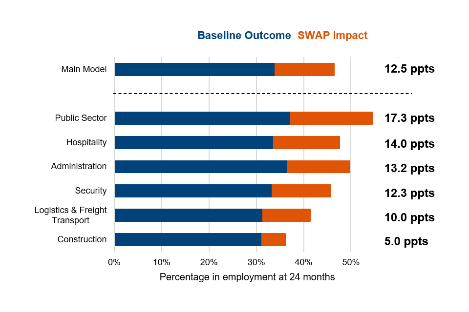
SWAP sector	Baseline Outcome: % in employment at 24 months	SWAP Impact: % in employment at 24 months
Main Model	34%	13%
Public Sector	37%	17%
Hospitality	34%	14%
Administration	37%	13%
Security	33%	12%
Logistics and Freight Transport	31%	10%
Construction	31%	5%

References

Caliendo, M., Mahlstedt, R. and Mitnik, O. (2014) ‘Unobservable but unimportant? The influence of personality traits (and other usually unobserved variables) for the evaluation of labour market policies’, IZA discussion paper 8337

Cann, J. (2024) ‘Kickstart Scheme: A Quantitative Impact Assessment’, Department for Work and Pensions

Coleman, N., Hingley, S. and McGinigal, S (2013) ‘Employer perceptions of work experience and sector-based work academies’, Department for Work and Pensions

Department for Work and Pensions (2024), ‘Get Britain Working Analytical Annex’

Department for Work and Pensions (2024) ‘Sector-based Work Academy Programme: qualitative case study research’

Department for Work and Pensions, ‘Sector-based Work Academy Programmes (SWAPs) Management Information’

Fujiwara D. (2010) ‘The DWP Social Cost-Benefit Analysis framework (WP86)’, Department for Work and Pensions

Haigh, R., Ward, R. and Woods, J. (2016) ‘Sector-based work academies: a quantitative impact assessment’, Department of Work and Pensions

Hillmore, A., Marlow S. and Ainsworth P. (2012) ‘Impacts and Costs and Benefits of the Future Jobs Fund’, Department for Work and Pensions

HM Treasury (2022) ‘The Green Book: appraisal and evaluation in central government’

HM Treasury (2011) ‘The Magenta Book – GOV.UK’

Kay, J. and Marlow, S. (2020) ‘The Work Programme: A quantitative impact assessment’, Department for Work and Pensions

1. Fujiwara D. ‘The DWP Social Cost-Benefit Analysis framework (WP86)’ Department for Work and Pensions working paper 86, 2010. ↩

2. Sector-based Work Academy Programmes (SWAPs) Management Information ↩

3. Sector-based work academies: a quantitative impact assessment – GOV.UK ↩

4. Sector-based Work Academy Programme: qualitative case study research – GOV.UK ↩

5. Microsoft Word - Impacts and costs and benefits of the FJF_final.doc – GOV.UK ↩

6. The Work Programme: A quantitative impact assessment – GOV.UK ↩

7. Kickstart Scheme: A Quantitative Impact Assessment – GOV.UK ↩

8. The Magenta Book – GOV.UK ↩

9. Unobservable, but Unimportant? The Influence of Personality Traits (and Other Usually Unobserved Variables) for the Evaluation of Labor Market Policies – (iza.org) ↩

10. Variables from the LEO dataset and variables from the LILR dataset are used for matching in separate models. ↩

11. We may be undercounting the number of individuals from both the treatment and comparison groups who are earning by not including in the number of individuals earning those who had earnings from self-employment, but no payslip earnings recorded. ↩

12. The percentage point impact in each month is multiplied by the number of days per month. These monthly estimates are then summed together to create an overall estimate for the 24-month period ↩

13. Get Britain Working White Paper – GOV.UK ↩

14. While 8.1 ppts is still a high additional employment impact, this is low relative to the main model impact and the other subgroups shown in chart 3.7. ↩

15. See Appendix A for a list of variables used from the LEO dataset ↩

16. See Appendix A for a list of variables used from the LILR dataset. ↩

17. The Green Book (2022) – GOV.UK ↩

18. This cost per start was found by dividing the total amount of AEB spend on the programme (approximately £22m) by the number of SWAP participants reported to have taken part in AEB funded training. ↩

19. The DWP Policy Simulation Model is a microsimulation model which combines data from the Family Resources Survey with information on the UK tax and benefit systems. This allows users to estimate the changes in benefit payments and tax revenue that occur when unemployed individuals with a given set of characteristics move into work. ↩

20. In order to estimate increases in indirect tax revenue, Office for National Statistics estimates of indirect tax burdens were applied to estimates of participants’ disposable income obtained from the DWP Policy Simulation Model. ↩

21. For a thorough discussion of the non-monetised costs and benefits of employment programmes, see Fujiwara (2010). ↩

22. Fujiwara (2010) presents evidence of a causal relationship between individuals’ income levels and their propensities to commit acquisitive crime. ↩

23. Members of society generally prefer to receive goods and services sooner rather than later. In order to take account of this ‘social time preference’, costs and benefits which occurred in ‘future’ periods have been discounted in line with the methodology prescribed in the HM Treasury Green Book. For a detailed description of this methodology, see HM Treasury (2022). ↩

24. See, for example, Coleman et al (2013) – Employer perceptions of work experience and sector-based work academies. ↩

25. An individual is considered to have a current disability if they are recorded as having a restricted ability to work and a live fit note at the time of the SWAP start/pseudo start date. ↩

26. Rubin’s B and R summarise the covariate balance of the sample. Rubin’s B measures absolute difference in the mean propensity scores between the treatment and comparison group and should be under 25 to satisfy a balanced sample. Rubin’s R measures the ratio of treatment to comparison variances of the propensity scores and should be between 0.5-2 to satisfy a balanced sample. ↩

27. The main model result has still been included in Chart C.1 for reference. ↩

28. Sector-based Work Academy Programmes (SWAPs) Management Information – GOV.UK ↩