Research and analysis

Impact evaluation of the European Social Fund 2014-2020 programme in England

Published 14 February 2025

Applies to England

DWP research report no. 1087

A report of research carried out by the Department for Work and Pensions. Crown copyright 2025.

You may re-use this information (not including logos) free of charge in any format or medium, under the terms of the Open Government Licence.

To view this licence, visit the National Archives

Or write to:

Information Policy Team
The National Archives
Kew
London
TW9 4DU

Email: psi@nationalarchives.gov.uk

This document/publication is also available on our website at: Research at DWP

If you would like to know more about DWP research, email socialresearch@dwp.gov.uk

First published February 2025.

ISBN 978-1-78659-798-4

Voluntary statement of compliance with the Code of Practice for Statistics

The Code of Practice for Statistics (the Code) is built around 3 main concepts, or pillars, trustworthiness, quality and value:

• trustworthiness – is about having confidence in the people and organisations that publish statistics
• quality – is about using data and methods that produce assured statistics
• value – is about publishing statistics that support society’s needs for information

The following explains how we have applied the pillars of the Code in a proportionate way.

Trustworthiness

This analysis has been conducted by professionally badged analysts in the Department for Work & Pensions. The methodology used for the impact analysis is based on recommendations in the published ESF European Social Fund impact evaluation: research design and scoping study which was conducted by an independent research company Ecorys.^{[footnote 1]} The methodology has also been additionally assured by both external and internal experts in the application of these techniques to labour market programmes.

Quality

This analysis has been carried out using established Propensity Score Matching and Difference-in-Difference methods to measure a counterfactual. This approach is based on recommendations from internal and external experts in the field of evaluating labour market programmes. Cost Benefit Analysis uses the published DWP Social Cost Benefit Analysis Framework.^{[footnote 2]} The final analysis and report have been through the Department’s rigorous quality assurance process and findings have been shared with senior programme governance through the European Social Fund in England’s Growth Programme Board.

Value

This research provides robust evidence of the impact and value for money of the European Social Fund 2014-2020 programme in England. Used alongside other published evidence from the programme evaluation^{[footnote 3]} it forms a legacy that is and will be used to inform the development of current and future domestic employment and skills programmes, particularly those supporting people experiencing barriers to labour market participation.  

Executive Summary

Background

This report presents an impact assessment and accompanying cost benefit analysis of the ESF programme in England that was funded between 2014-20. Programme activity began in 2015 and continued through to 2023, despite the name. In this analysis the data includes those that started on ESF between 2015 and 2020, in order to allow time for three-years post-start outcomes to accrue.

ESF is a large voluntary programme. Participants have to be aged 15 and above at the start of the programme and can be unemployed, employed, or inactive. Some participants are in education when they start on the programme and some may be care-leavers, single parents and either be in, or just being released from, prison.

ESF provides a wide range of support that is often personalised, facilitated by a key-worker and links the participant to a range of services to meet their individual needs, or so called “wrap-around” support. There are a significant number of providers, operating on a grant funding basis spread across England.

Methodology

The impact assessment looks at labour market outcomes for participants on ESF who started after 2015 and for whom we have enough data to monitor their outcomes for three years post-start. These outcomes measure whether, and for how long, people were on benefits and employed. The outcomes for those who started on ESF were compared to people not on ESF who shared similar characteristics. This average treatment effect on the treated allows us to measure the impact of ESF.

Individuals in the two groups are matched with one another using a Propensity Score Matching (PSM) approach. This uses a significant amount of data to look at characteristics that are then used to assign a score - the probability of an individual participating in the programme. We then match people with similar scores on these observed characteristics in an attempt to eliminate any bias that would exist if we just matched on individual characteristics, this matching process is a strength of a PSM approach. There is a risk that bias remains for characteristics that cannot be observed, but by using substantial amounts of data the aim is to minimise that risk.

This analysis tracks labour market outcomes for three years, whilst we also present intermediate impacts at years 1 and 2. Analysis has attempted to quantify the 4- and 5-year impact, but the results have not yet been robust enough to present in this analysis owing to smaller sample sizes. These results are then used to produce a cost benefit analysis. This focuses on estimating the cost effectiveness of ESF from the point of view of the exchequer (i.e. a narrow view of direct costs and benefits that are part of DWP’s remit) and society (which accounts for economic output). This analysis follows the DWP Social Cost-Benefit Analysis framework (Fujiwara, 2010^{[footnote 4]}). This approach is consistent with various other analyses produced by DWP.

Key Findings

• This analysis provides evidence that participating in ESF statistically increases time in employment and reduces time spent on inactive benefits for example ESA , and increases time spent on active benefits^{[footnote 5]} for example UC.
• We estimate that, on average, ESF participants spend around 39.7 more days in employment in the three years post-start compared to had they not participated in ESF.
• Those who start the programme already employed spend an additional 29.7 days in employment, after three years, compared to had they not participated in ESF.
• Those who start ESF when unemployed spend an additional 34.2 days in employment, after three years, compared to had they not participated.
• Those who start ESF when inactive spend an additional 76.0 days in employment, after three years, compared to had they not participated.
• These impacts accrue, increasing year-on-year, to reach the quoted figures after three years and remain above zero even at the three-year point.
• For the exchequer ESF makes a return of £0.69 for every pound spent at three years (i.e. a net loss). This is largely due to the relatively narrow scope of exchequer benefits in this context that do not include non-DWP outcomes such as education and criminal justice. This is when the benefits are compared to the ESF costs of delivering the programme.
• ESF makes a return of £1.50 for every pound of spend when looking at the societal perspective, which included increases in economic output.

Acknowledgements

This report and the several years of analysis that have gone into it, has been part-funded by European Social Fund Technical Assistance money. This money was used to commission external experts in the field of labour market evaluation to assure the methods used in the analysis. We would like to thank Dr Sergio Salis (ICF) and Dr Stefan Speckesser (University of Brighton) for their contributions.^{[footnote 6]} We would also like to thank staff at IFF Research and Ecorys for their contributions to the wider ESF evaluation programme, of which this work is a culmination. 

A number of DWP labour market analysts have contributed to this analysis over several years for which we are grateful. This includes Alexander McPhie, Mike Oldridge, Ryan Davison, Luke Montgomery, David Wynne, Alicia Slater, Zana Wellicome, Thea D’Ambra, John Gregson, Katelin Archer and Charlie Kitson. We are also grateful for the advice and assurance of the DWP Employment Data Lab team including Luke Barclay, James Crowe and Ryan Bagnall.

Finally, we would like to thank and acknowledge our colleagues in the ESF Managing Authority and the hundreds of ESF projects who have provided the data for the analysis, without which this evaluation would not have been possible.

Adam Robinson and Nick Campbell ESF Analysis and Evaluation Leads Department for Work and Pensions September 2024

Author details

This report has been authored by members of the ESF Evaluation and Analytical teams based in the Labour Market Analysis Division of DWP. Many individuals, named in the acknowledgements, have made key contributions towards this report. These teams have existed since the start of the programme to provide analytical support to the Managing Authority and a functionally separate evaluation of the 2014-2020 programme. This report is the final one in a series of published evaluations available on gov.uk including the Youth Employment Initiative process and impact evaluations, a scoping and feasibility study informing the methods and analysis in this report, a qualitative case study report and two leavers survey reports covering the first and second half of the programme.^{[footnote 7]}

Glossary of terms

Term	Definition
Active Benefits	Benefit for people who are actively looking for work, including Universal Credit Employed, Job Seekers Allowance and Universal Credit Unemployed.
Co-Financing Organisations (CFOs)	Public bodies which bring together ESF and domestic funding for employment and skills so that ESF complements national programmes. Provision for the 2014-2020 Operational Programme was delivered through four  Co-Financing Organisations, the Education and Skills Funding Agency (ESFA), DWP, National Lottery Community Fund (formerly Big Lottery Fund); His Majesty’s Prison and Probation Services (HMPPS, formerly the National Offender Management Service or ‘NOMS’), as well as intermediary and devolved bodies (Greater London Authority, Greater Manchester Combined Authority, West of England Combined Authority) and Direct Providers.
Common support/On support/Off support	Once propensity scores have been assigned for each observation, the overlap of propensity scores between the participants and comparison group is called ‘common support’. Those who fall in the overlap are referred to as ‘on support’, those who do not fall into the overlap are ‘off support’.
Comparison group	Carefully selected subset of the comparison pool, selected to have outcomes as similar as possible, to act as a counterfactual.
Conditional Independence Assumption	CIA requires variables that affect treatment assignment and treatment outcomes be observable.
Counterfactual Impact Evaluation	CIE is a type of impact evaluation using a counterfactual analysis approach. Counterfactual analysis compares the real observed outcomes of an intervention with the outcomes that would have been achieved had the intervention not been in place (the counterfactual). A CIE can involve use of a randomised controlled trial (RCT) methodology, also referred to as an ‘experiment’, or quasi-experimental methods that seek to mimic an experiment, often through construction of a comparison group to compare outcomes with the treatment group receiving an intervention. The CIE for the European Social Fund impact evaluation uses a quasi-experimental approach.
Difference in Difference (DiD)	DiD analysis is an impact evaluation technique, seeking to estimate the effect of a treatment on an outcome of interest through assessing change over time in an outcome for a treatment group relative to the average change over time for a control/comparison group.
Employed	Claiming Universal Credit (UC) with conditionalities earning enough or light touch in work
European Social Fund (ESF)	The European Social Fund (ESF) is the European Union’s main fund for supporting employment in the member states of the European Union as well as promoting economic and social cohesion.
ESF provider	Refers to any or all organisations delivering ESF funded provision, including CFOs, opt-in organisations, direct bid providers, and intermediary bodies or organisations contracted by them to offer provision.
Inactive	Claiming Employment Support Allowance (ESA) or UC with conditionalities no work-related requirements, work preparation of work focused interview
Inactive Benefits	Benefit for people who are not actively looking for work including Employment Support Allowance and Universal Credit Inactive.
Jobless household	Jobless households are households where no member is in employment, i.e. all members are either unemployed or inactive.
Participant Group	The people who took part in the programme being evaluated.
Programme Propensity Score Matching (PSM)	The employment support provision under investigation. PSM is a statistical technique used to estimate the impact of an intervention on a set of specific outcomes. It mimics an experimental research design by comparing outcomes for a treatment group and a statistically generated comparison group, which is similar to the treatment group in its composition.
Pseudo-start date	Dates assigned to the comparison pool in lieu of the real programme start dates of the participant group.
Rubin’s B & R	A test used to evaluate the matching in PSM.
Statistically significant	Describes a result where the likelihood of observing that result by chance, where there is no genuine underlying difference, is less than a set threshold. In this ESF report, this is set at 5%.
Unemployed	Claiming Job Seekers Allowance (JSA) or UC with conditionalities intensive work search or light touch out of work
Youth Employment Initiative (YEI)	The Youth Employment Initiative (YEI) is one of the main EU financial resources to support Youth Guarantee schemes.3 The initiative was launched to provide support living in regions where youth unemployment was higher than 25 per cent. It ensures that in parts of Europe where the challenges are most acute, young people can receive targeted support. In England the YEI was aimed at 15-29 year old NEETs (Not in Employment, Education or Training).

Abbreviations

Acronym	Definition
ATT	Average effect of Treatment on the Treated
CBA	Cost Benefit Analysis
CBR	Cost Benefit Ratio
CFO	Co-Financing Organisation
CIA	Conditional Independence Assumption
CIE	Counterfactual Impact Evaluation
DiD	Difference-in-Differences
DWP	Department for Work and Pensions
ESA	Employment and Support Allowance
ESF	European Social Fund
ESFA	Education and Skills Funding Agency
ESIF	European Structural and Investment Funds
EU	European Union
HMPPS	His Majesty’s Prison Probation Service
HMRC	His Majesty’s Revenue and Customs
IP	Investment Priority
IMD	Index (or indices) of Multiple Deprivation
JSA	Jobseeker’s Allowance
MA	Managing Authority
MI	Management Information
NBD	National Benefits Database
NLCF	National Lottery Community Fund
NEET	Not in Education, Employment or Training
NINo	National Insurance Number
PA	Priority Axis
PSM	Propensity Score Matching
SCBA	Social Cost Benefit Analysis
UC	Universal Credit
UCE	Universal Credit Employed
UCI	Universal Credit Inactive
UCU	Universal Credit Unemployed
UK	United Kingdom
YEI	Youth Employment Initiative

Summary

Introduction (Chapter 1)

What is ESF?

The European Social Fund (ESF) was set up to improve employment opportunities in the European Union (EU) and thereby raise standards of living. The Department for Work and Pensions is the Managing Authority (MA) of ESF funds in England.

The ESF 2014-20 Operational Programme – part of the European Structural and Investment Funds (ESIF) Growth Programme for England – aimed to deliver against priorities to increase labour market participation, promote social inclusion and develop the skills of the potential and existing workforce. As set out in the UK’s Withdrawal Agreement with the EU, the ESF programme continued to invest in projects after the transition period for leaving the EU ended on 31 December 2020, but all funding needed to finish by the end of 2023.

The programme is structured around 5 Priority Axes (PAs) based on the EU’s Thematic Objectives. This evaluation focuses on two of these:

• PA1: Inclusive Labour Markets
• PA2: Skills for Growth

Provision for the 2014-20 Operational Programme was delivered through four Co-Financing Organisations: the Education and Skills Funding Agency (ESFA); DWP; National Lottery Community Fund (NLCF); His Majesty’s Prison and Probation Services (HMPPS); Greater London Authority acting as an intermediary body with other organisations such as Greater Manchester Combined Authority having similar status, as well as Direct Providers (i.e. projects which bid directly to the Managing Authority).

Purpose of this analysis

This report evaluates the labour market impact of the European Social Fund (ESF), covering all ESF participants from 2015 to 2020, allowing for a three-year outcome tracking period.

The study centres on participants’ benefit receipt and movement into employment as outcomes. It does not attempt to estimate impact on educational outcomes, earnings or other outcomes that may result from ESF as DWP are still in the process of developing a robust way to estimate these with the data DWP currently holds. It does however include a cost benefit analysis of the labour market component.

The analysis follows recommendations from prior scoping studies by using Propensity Score Matching (PSM) and Difference-in-Difference (DiD) methodologies. The scoping studies did also recommend sub-group analysis, but we have not followed these recommendations as the data does not allow us to conclude why there may be differences between sub-groups.

This report contributes to the existing ESF evidence base of reports, including a leavers survey covering the 2016-2019 and 2021-2023 periods, as well as a qualitative evaluation published in 2022 and an impact analysis of the Youth Employment Initiative (YEI). Several other evaluations have also been published by external organisations.

Analytical Approach (Chapter 2)

Drawing of the Treatment Group

The treatment group is drawn from ESF administrative data which doesn’t contain national insurance numbers (NINos). To obtain NINos, DWP employs a two-step “fuzzy-match” process, which is explained in detail in the chapter, using participant contact details. This process is successful for just over half (52%) of ESF participants. The treatment group is restricted to participants who participated in an ESF programme in England, who are aged 19-64, who started on or before September 2020 and who were claiming benefits when they started on ESF. These ages allow us to track for months pre-start for even the youngest and cut off at retirement age for many. This aligns with other impact analyses. Participants are grouped depending on the type of benefit they were claiming at the start – employed, unemployed and inactive. The resulting treatment sample is 201,700.

Our treatment participant group differs slightly from the overall fuzzy-matched ESF participant group in several characteristics. Treatment participants are slightly younger, with a higher proportion under 25 (37% vs. 33%), and a slightly lower rate of disability (21% vs. 23%) and ethnic minority representation (23% vs. 26%). More treatment participants have lower educational attainment (22% vs. 17%) but are less likely to be homeless (1% vs. 4%) or from a jobless household (22% vs. 29%). Whilst there are minor differences between the two groups, we do not consider them large enough to materially affect the estimated impacts, particularly once we have controlled for the relevant characteristics.

Details of how the comparison pool is drawn can be found in Appendix 4.

Overview of Methodology

For the analysis, non-participants drawn from DWP data are assigned pseudo-start dates that mirror the distribution of participant start dates. Individuals are then tracked for three years post-(pseudo)start, with monthly flags indicating whether they had a live spell on employed, unemployed or inactive benefits or in PAYE employment. These flags are needed for the propensity score matching process, reducing processing time while maintaining match quality. The three-year tracking periods allows sufficient time for some outcomes to accrue, while maintaining a large enough sample size. Though it is also limited to three years due to the data available at the time.

We estimated the average effect of the ESF employment programme on participants using propensity score matching (PSM). PSM creates a comparison group of non-participants who share key characteristics with participants. This enables us to estimate what a participant’s labour market outcomes would have been without the programme (the counterfactual). By matching participants and non-participants based on their propensity scores, PSM helps reduce the impact of confounding variables and selection bias, mimicking a randomised control trial (RCT). RCT approach was not feasible due to the way the ESF programme was managed and operated, whereby the European Commission want to maximise uptake of support. The effectiveness of PSM relies on the Conditional Independence Assumption (CIA) being met. The CIA states that, after controlling for a set of variables, assignment to ESF is independent of the outcomes. Whilst this is challenging to achieve in voluntary programmes where unobservable traits like motivation play a role, the method used should allow these characteristics to be controlled for by use of a rich dataset.

In this analysis, we also use difference-in-differences (DiD) approach, comparing labour market status of ESF programme participants and non-participants before and after the programme. This method assumes that, without intervention, both groups would have followed the same outcome trends both pre- and post-treatment, known as the common trend assumption and that only the treatment causes a difference in outcomes. While the voluntary nature of the programme could potentially violate this assumption – since participants might be more motivated – the nature of the analysis will mean that we control for this as much as possible.

Treatment and Comparison Groups

Across the three groups of benefit recipients – employed, unemployed and inactive – those in the treatment group generally appear more disadvantaged compared to non-participants in the comparison group and tend to have higher rates of disability, a greater proportion of ethnic minorities, and are often male. They also typically spent longer on benefits before joining the programme. These trends suggest that individuals who participate in the ESF programme face higher barriers in the labour market than those who did not participate, regardless of the type of benefits they received.

Limitations

Due to the lack of National Insurance Numbers (NINos) in the programmes data collection, a fuzzy match process was used to retrieve these, in order to access data on participants’ benefit and employment histories. However, this was only successful for about half (52%) of the participants. As a result, the treatment group is limited to participants with successful NINo matches and further narrowed to those claiming benefits at the start of the ESF provision. This ensures there is sufficient data for the analysis, but it means the results may not represent all participants, as just over a third (35%) of the those for who NINos were generated for were on benefits when they began ESF programme.

Another potential limitation is contamination of the control group, whereby non-identified participants on ESF for whom we do not have a NINo are present. Some efforts to exclude potential participants are included in our approach but we cannot verify how many may be in the control. If this was significant it could bias the results, potentially reducing the observed effect.

PSM was chosen as the most appropriate method to evaluate the ESF programme based on a feasibility report and the voluntary nature of participation.  The PSM attempts to control for unobserved differences, which may bias the analysis, but we cannot estimate in which direction or to what degree. The expectation is by having a rich amount of data, we can control for enough observable characteristics that will render the unobserved ones immaterial and to such an extent that this does not violate the independence assumption.

Results (Chapter 3)

Outcomes of Propensity Score Matching

The quality of the propensity score matching process is assessed by checking the “common support”, which indicates the proportion of treatment group observations that have suitable matches in the comparison group based on the closeness of propensity score, as defined by a calliper of 0.0001. Observations without a match, known as “off support”, are excluded from that particular sub-group analysis. For the employed, unemployed and inactive benefit groups, the vast majority were on support, with a match found for at least 96% of the observations in each treatment sample.

Findings from Impact Analysis

A key result across all three benefit groups is that ESF participants are more likely to be in or remain in employment in the three years post programme start than had they not participated on the programme. These results are all statistically significant.

The ESF programme had a positive impact on employment outcomes for the employed benefit group (i.e. those employed and claiming benefits). Overall, these participants are likely to spend 30 additional days in employment over the three years following participation compared to non-participants.

Similarly, the programme also had a positive impact on employment outcomes for the unemployed benefit group, with these participants likely to spend 35 additional days in employment over the three years following participation compared to non-participants.

The analysis showed ESF had a positive impact on employment outcomes for the inactive benefit group, suggesting participation substantially increased an individual’s chances of being in employment over the three-year tracking period. These participants were likely to be in employment for an additional 76 days compared to non-participants.

The ESF programme increased time on employed and unemployed benefits over the three-year tracking period, meaning participation increased an individual’s chances of being on these types of benefits over this period. This means participants move into the labour market, or are closer to the labour market, than they would have been in the absence of ESF.   

Universal Credit differs from previous benefits, in that it is entirely possible for someone to remain on UC whilst entering employment. UC is an income-related benefit therefore employment and benefit receipt can coexist, subject to the individual’s income level, unlike under for example, JSA which stopped once someone entered employment. Movement into employment, whilst still being on benefit, is still a positive impact both for the individual and the exchequer compared to just receiving benefit alone.

Overall, employed benefit participants are likely to spend 27 additional days on benefits and unemployed benefit participants are likely to spend 140 additional days on benefits across the three years compared to non-participants. However, participants in these benefit groups are also more likely to be in employment following participation compared to those who did not participate. It is likely they are moving into employment with the support of Universal Credit. Inactive benefit participants spent 20 fewer days on average in receipt of benefits across the three years compared to non-participants.

Understanding from Differing Impacts

The ESF programme’s impact varies across benefit groups, with the most pronounced effect observed among inactive benefit recipients, who are typically further from the labour market. However, other groups also obtained positive outcomes, mostly in the form of additional time in employment.

The size of the impacts were different across each of these groups. Causal factors are difficult to isolate in this type of analysis, although some suggested factors include the participants’ relative labour market starting point as well as the type of provision they received on ESF could influence the relative differences.

The sharp initial rise in benefit receipt following the start of ESF provision across all groups may be explained by the programme ‘lock-in’ effect. This can delay participants’ transition away from benefits as they continue to engage with the programme, seeking better job outcomes. Participants also report increases in softer outcomes such as enhanced skills, confidence and motivation evidenced by survey data, which may lead to prolonged job searches as participants set higher job expectations. Although, we cannot compare these with a counterfactual.

Cost Benefit Analysis (Chapter 4)

Social Cost Benefit Analysis Methodology

On average, participants spent an extra 40 days in employment over 36 months compared to similar individuals who did not participate. The impact varied based on initial labour market status: those on inactive benefits had the greatest employment impact with 76 days of additional employment, while unemployed participants had 34 additional days and those already employed when starting ESF gained 30 additional days.

The Social Cost Benefit Analysis (SCBA) evaluates ESF’s costs and benefits from two perspectives: the Exchequer and Society. The Exchequer perspective focuses on direct fiscal effects, like taxes and social security expenditure. While the Social perspective considers broader outcomes like employment output, travel costs, childcare and healthcare benefits. The resulting Cost-Benefit Ratio (CBR) shows the balance between the costs and benefits, with a ratio above £1:£1 signalling a positive return on investment.

The SCBA outlines the benefits of ESF participants moving into employment, including increased economic output, reduced operational costs, decreased reliance on benefits, higher tax revenues and reduction in healthcare costs. On the cost side, the calculation of CBR uses a flat unit cost, specific to the treatment group participants, aggregated from different ESF projects. We only focus on the additional costs of ESF for the treatment group. Other costs, such as other programme costs, could accrue to either participants or non-participants. Our analysis indicates that the proportions this apply to are relatively small and similar between the treatments and control groups and therefore are not required to be accounted for.

Social Cost Benefit Analysis Findings

At the three-year tracking point, the CBR is below £1 for the exchequer but above £1 for the social for the ESF programme. From the exchequer’s perspective, which only considers taxes and benefits related to employment, the benefits do not outweigh the costs, resulting in a net loss of £720 and a CBR of £0.69 for the programme. However, from a social perspective, the benefits outweigh the costs, generating a £1,160 surplus to society and a CBR of £1.50 for the programme.

The programme’s benefits increase over time as more outcomes are realised and more people complete provision, obtain outcomes and more data becomes available. The CBR is low at the 12-month point because many outcomes take time to accrue. It significantly improves after 24 and 36 months as more people see the impact of ESF. The analysis suggests that the positive impacts of ESF extend beyond the three-year tracking period. The difference between the treatment and non-treatment groups at the 36-month point is not zero, indicating that impacts are still present and therefore additional outcomes could be achieved if data were available for 48+ months. Whilst some early cohorts have reached that point, the sample size is too small to make a meaningful estimate in this report.

Our analysis also suggests that to “break even” on the exchequer savings, around 52 days of additional employment would need to be detected in the impact. At the current rates, if the three-year impact was sustained, we’d expect this to be achieved if we could track for four years.

Social Cost Benefit Analysis of Differing Groups

The analysis has focused on participants who are on benefits upon starting ESF. However, unlike other labour market programmes the characteristics of our participants varied. ESF includes individuals who may have been on UC as well as legacy benefits upon starting, unlike other programmes where all participants are on a single benefit. The analysis examines the impact between conditionality types, specifically comparing those who are unemployed, inactive and employed when they started ESF. This approach helps show a range of potential CBR estimated without creating unlikely scenarios.

The cost benefit analysis findings indicate that the impact is greatest for the inactive group, which aligns with ESF’s core purpose of helping those furthest from the labour market. The unemployed group shows the next highest impact, while the employed group has the lowest. Caution is advised in interpretating these results as definitive evidence of ESF’s effectiveness for one group over another, given the different characteristics and outcomes across groups.

Conclusions (Chapter 5)

Impact Analysis

The analysis estimated the impact of the ESF programme on participants using the average treatment effect on the treated (ATT) through Propensity Score Matching (PSM). By comparing outcomes of ESF participants and a similar non-participant group, both on benefits at the start, we aim to estimate the programme’s effect. Participants are split into groups based on the type of benefits they are claiming on starting, whether they are employed, unemployed or inactive. The primary outcome is employment, with ESF participants spending around 40 days more in employment over the three-year period than non-participants. While ESF is voluntary, we do attempt to control for unobservable characteristics and sensitivity analysis has been carried out to ensure the robustness of our estimates. Overall, ESF has the effect of increasing the likelihood of participants gaining employment.

Cost Benefit Analysis

A Cost Benefit Analysis (CBA) was conducted using the impact analysis results to assess the cost-effectiveness of the ESF programme over one, two and three years, both from exchequer and societal perspectives. At the three-year mark, for every pound invested, the exchequer benefits by £0.69 and society by £1.50, with sensitivity analysis confirming the robustness of these results. The analysis also revealed that while employed participants see lower returns, those unemployed or inactive at the start experience greater benefits. Beyond three-years the positive benefits are likely to persist, given that the net impact is above zero at the three-year point. These results broadly align with the previously published YEI impact estimates and CBA figures. Though potential costs and benefits such as health and crime related impacts were not included due to lack of data.

Chapter 1: Introduction

This chapter briefly describes the European Social Fund programme in England and explains the purpose of this analysis, including how it fits with other parts of the evaluation programme

What is ESF?

1.1 What is the European Social Fund?

The European Social Fund (ESF) refers to ESF in England during the programming period 2014-2020. It was set up to improve employment opportunities in the European Union (EU) and thereby standards of living. The Department for Work and Pensions is the Managing Authority (MA) of ESF in England. The Devolved Administrations have their own separate ESF programmes, which are administered locally and have their own evaluations.

The ESF 2014-20 Operational Programme - part of the European Structural and Investment Funds (ESIF) Growth Programme for England - stated that the aims of the programme were to deliver against priorities to increase labour market participation, promote social inclusion and develop the skills of the potential and existing workforce. As set out in the UK’s Withdrawal Agreement from the EU, the ESF programme continued to invest in projects after the transition period for leaving the EU ended on 31 December 2020, but all funding needed to finish by the end of 2023. 

The programme is structured around 5 Priority Axis (PAs) based on the EU’s Thematic Objectives. This impact evaluation focuses on two of these:

• PA 1: Inclusive Labour Markets
• PA 2: Skills for Growth

The other three PAs do not focus on labour market outcomes, and therefore no participants are included in the analysis.

Provision was delivered through 4 Co-Financing Organisations, the Education and Skills Funding Agency (ESFA), DWP, National Lottery Community Fund (NLCF, formerly the Big Lottery Fund) and His Majesty’s Prison and Probation Service (HMPPS, formerly National Offender Management Service). Greater London acts as an intermediate body, with some powers of the MA devolved to them as do some other organisations such as Greater Manchester Combined Authority. The remaining funding is delivered through Direct Bid providers which are projects that bid directly to the Managing Authority for funds.

1.2 Purpose of this analysis

The analysis in this report aims to provide a quantitative assessment of the impact of the labour market element of ESF. Although the study is published by DWP, it is in its capacity as MA of the whole programme, therefore all participants are in scope for the analysis. Due to data limitations the predominant focus is on benefit receipt and movement into employment as outcomes for participants.

The study does not attempt to estimate the impact on educational outcomes, earnings or other outcomes that may result from ESF even though they are all part of the programme’s targets. This is largely due to a lack of robust method with existing data for estimating these impacts existing at this point.

Also, due to the timing of this analysis we only use participants who started in the programme from the start of the programme in 2015 to 2020. This is to allow sufficient time post-start, or pseudo-start^{[footnote 8]} in the case of the comparison group, to track outcomes for three years and to allow the data to settle.

The programme covered the main phase of roll-out of Universal Credit, as a result, the study covers both legacy (for example JSA, ESA) and Universal Credit benefits as control factors as well as outcomes.

This study also includes a cost benefit analysis of the overall cost effectiveness of the labour market only element of the programme, this is presented in section 4.

The Department published two scoping studies on how it may be possible to undertake impact analysis. One looked at what was possible for YEI^{[footnote 9]} as well as one that looked at ESF as a whole^{[footnote 10]}. This paper follows many of the recommendations of the scoping study in terms of the approach used; most notably using Propensity Score Matching (PSM) and Difference-in-Difference (DiD) approaches. It stops short of subgroup analysis for the reasons laid out in the scoping study around overlap.

This paper is not the first to cover what ESF has achieved; several reports have already been published that build the ESF evidence base. These reports take many forms, including early impacts of ESF covering 2007 to 2013^{[footnote 11]}, a leavers survey covering the 2016-2019 period has already been published^{[footnote 12]}, as well as a leavers survey covering 2021-2023. A qualitative evaluation^{[footnote 13]} was also published in 2022 alongside an impact analysis that looked at only the YEI portion of the programme^{[footnote 14]}.

Several other evaluations have been published by organisations such as NLCF^{[footnote 15]} and DWP in their previous guise as CFO for the 2007-13 ESF programme^{[footnote 16]}.

Chapter 2: Analytical approach

This section presents the analytical approach for the impact analysis of the European Social Fund (ESF) for participants who started ESF after 2015, for the three-year period after they started the intervention. The drawing of the treatment group is set out in section 2.1. The methodology is set out in section 2.2 with figures for who is in our treatment and comparison groups in section 2.3. The limitations of our approach are discussed in section 2.4.

The aim of this evaluation is to compare those who went on ESF provision and assess their outcomes with a matched group who did not participate. Our analysis looks at ESF as a complete programme, we do not currently split the data into project level^{[footnote 17]}.

2.1 Drawing of the Treatment Group

A key feature of ESF provision is that it is available to anyone in England with disadvantages, regardless of their labour market status or prior interaction with the benefits system. This broad eligibility leads to a greater heterogeneity of participant characteristics that is often not seen by other DWP employment programmes where the eligibility criteria is more defined.

We describe below the method used for drawing the treatment group being evaluated and their basic characteristics.

2.1.1 Who are the Treatment Group

Our treatment group is drawn from ESF administrative data which is essentially a census of all participants. This data is comprised of Management Information (MI) collected by the Managing Authority (MA) from all ESF funded projects containing information about characteristics, outcomes and skill-levels. However, it does not contain any common personal identifiers i.e. National Insurance Numbers (NINo). NINos are used to link to DWP administrative data in order to gain an understanding of participant benefit and employment histories.

Therefore, DWP use a “fuzzy-match” process to obtain NINos. The matching process occurs in two steps, both undertaken by a small, specialised team as access to this data is tightly controlled. In the first step, the ESF MI is linked to the ESF participant contact details database to obtain details needed for fuzzy matching. The second step is where the fuzzy match is performed to link the contact details we do have to the department’s customer information system (CIS) and obtain the NINos. CIS database is searched for a customer record with a surname, postcode, date-of-birth and gender that corresponds to the record in the MI and contact details. Approximately 52% of ESF records are assigned a NINo in this way, with the remaining 48% not matching for a variety of reasons. For example, failure to match at the first stage is most likely because the organisation leading the project did not provide participant contact details; failure to match at the second stage could be due to lack of information in the contact details provided or discrepancies between details recorded in the contact details database and the CIS database. The limitations of this process are discussed further in Section 2.4.

Following this process, our treatment group is restricted to participants meeting the conditions set out below:

• those who participated in an ESF programme in England
• those aged 19-64, in order to track some benefit history before ESF start date
• those who started provision on or before September 2020, in order to track impacts for 3 years after start date
• those who were claiming benefits when they started ESF provision, in order to have a sufficient amount of data for the matching methodology we use

Participants are split into 3 groups depending on the type of benefit they were claiming within 30 days of their ESF start date. These groups described in Table 1 are determined by the benefit spells contained in the administrative data.

Table 1: Benefit claimant groupings

Group	Description
Employed	Claiming UC with conditionalities earning enough or light touch in work
Unemployed	Claiming JSA or UC with conditionalities intensive work search or light touch out of work
Inactive	Claiming ESA or UC with conditionalities no work-related requirements, work preparation or work focused interview

The resulting treatment sample size is 201,700 participants. This is comprised of 9,630 employed benefit claimants, 164,418 unemployed benefit claimants and 27,652 inactive participants.

2.1.2 How Representative is our Treatment Group

In this section we describe personal and demographic characteristics of ESF participants who we have a NINo match for and of all ESF participants in the MI. These are listed in the table below (Table 2).

Table 2: Summary statistics detailing personal and demographic characteristics of ESF matched participants and all ESF participants

	ESF Matched Participants	All ESF Participants
Observations	1,189,544	2,411,684

Personal / Demographic Characteristics

	ESF Matched Participants	All ESF Participants
Under 25 (%)	37%	33%
55+ (%)	9%	10%
Male (%)	54%	57%
Disabled (%)	21%	23%
Ethnic Minority (%)	23%	26%
Lone Parent (%)	7%	8%
Below Primary Education (%)	22%	17%
Homeless (%)	1%	4%
Jobless Household (%)	22%	29%
Unemployed (%)	44%	52%
Inactive (%)	16%	21%

The proportion of participants under 25 is slightly greater for matched participants (37%), compared with all participants (33%). There is little difference between matched ESF group and all ESF group in the proportion aged 55 and over (9% vs 10% respectively).

Over half of participants in both groups are male (54% and 57%) and there is a slightly higher rate of disability among the all ESF participant group (23%) than in the matched ESF participant group (21%). This is similar for the proportion of ethnic minorities (23% in matched vs 26% in all).

A greater proportion of all ESF participants (4%) than matched ESF participants (1%) are homeless. Similarly, those from a jobless household is higher among all ESF participants compared to ESF matched participants (29% vs 22% respectively).

More matched ESF participants (22%) than all ESF participants (17%) have a level of education which is below that of primary. Fewer matched ESF participants have an unemployed or inactive labour market status (44% and 16%), compared to all ESF participants (52% and 21%).

Despite the differences in characteristics, we conclude that the ESF participants we use in our analysis are representative of the ESF population as a whole.

2.2 Overview of Methodology

In this section, we outline the methodology used in our analysis to estimate the average effect on the ESF programme on its participants. We use a technique called Propensity Score Matching (PSM) which controls for observable differences in characteristics between groups. Our methodology relies heavily on the approach recommended in the scoping study. We employ similar techniques to that of other evaluations across the department, including Sector Based Work Academy (SBWA), the Employment Data Lab and Kickstart.

2.2.1 When Treated Started on ESF

Participation on the ESF programme began in March 2015. Figure 1, Figure 2 and Figure 3 shows the distribution of programme start dates between March 2015 and August 2020 for each benefit group.

The inflow of employed participants (Figure 1) increased from one participant starting in March 2015 to 155 participants starts in January 2017, before peaking at 345 per month in September 2018. In the two years between October 2018 and August 2020, participant inflows per month remained relatively steady from 255 participant starts in October 2018 to 261 participant starts in August 2020, with at least 100 participant starts each month in between. The number of participant starts reached cumulative total of 9,630 by the end of August 2020.

Figure 1: Monthly starts and cumulative starts on ESF for the employed treated group

The inflow of unemployed participants (Figure 2) increased from 13 participant starts in March 2015 to 2,541 participant starts six months later in September 2015, before peaking at 5,336 per month in May 2017. In the three years following June 2017, participant inflows per month steadily declined from 5,234 participant starts in June 2017 to 1,614 participant starts in August 2020. The number of participant starts reached cumulative total of 164,418 by the end of August 2020.

Figure 2: Monthly starts and cumulative starts on ESF for the unemployed treated group

The inflow of inactive participants (Figure 3) increased from 13 participant starts in March 2015 to 682 participant starts six months later in September 2015, before peaking at 973 per month in September 2017. In the three years between October 2017 and August 2020, participant inflows per month steadily declined from 626 participant starts in October 2017 to 323 participant starts in August 2020. The number of participant starts reached a cumulative total of 27,652 by the end of August 2020.

Figure 3: Monthly starts and cumulative starts on ESF for the inactive treated group

Non-participants in each benefit group are assigned a pseudo-start date (in lieu of an actual start date) in a way that matches the distribution of participant start dates in each benefit group. Further detail on pseudo start dates can be found in Appendix 2.

2.2.2 Use of monthly flags and tracking for two- and three-years post start

The outcome period covered for each individual spans from their ESF/pseudo start date to three years later. We track the benefit claims and employment spells for each individual in the 156 weeks post their ESF/pseudo start date. For each of these weeks, a flag is created to indicate whether or not the individual had a live spell on benefits or in employment in that week. These weekly flags are aggregated to provide us with monthly flags. The monthly flag is equal to one if the individual had a benefit or employment spell in at least one of the four weeks.

The flags are used as both control and outcome variables in the propensity score matching (PSM). They were created as a way to reduce the number of control variables used in the PSM which greatly reduced the processing time but had little impact on the quality of the match. It also guards against “overfitting” the model by having too many similar variables.

The length of time the analysis tracks for is a balance. The decision to use 156 weeks (three years) was taken as it allows time for outcomes to accrue, particularly when individuals on may be on ESF support for up to three years but not so long as to have few people have achieved that duration. The longer we track, then the fewer people will have reached that threshold and therefore the fewer in our sample. Three years seems to be an adequate balance at this point.

We are also currently limited to this period as our administrative data only extends to 2023. Therefore, individuals who started an ESF programme after 2020 cannot be monitored beyond three years.

2.2.3 Propensity Score Matching

To estimate the average effect of the ESF employment programme on its participants (average effect of the treatment on the treated, ATT) we use propensity score matching (PSM). PSM involves estimating the probability (propensity score) of an individual participating on the ESF programme given their observed characteristics.

The aim of PSM is to construct a comparison group of individuals who did not participate on the ESF programme and match with relevant characteristics to those who did. If this is successfully achieved, we can use the labour market outcomes of non-participants to estimate the labour market outcomes of participants, had they not participated in ESF provision. Another way of describing this is the “counterfactual” i.e. what would have happened to participants anyway, if ESF didn’t exist. It is likely some of the treated would have gained employment anyway, due to the dynamic nature of the labour market, so not every outcome achieved by ESF participants would be “additional”. This is covered more in 2.2.4.

Individuals in the treatment group are matched with individuals in the comparison pool based on their computed propensity scores, ensuring that the two groups are balanced i.e. comparable in terms of observed characteristics. If the PSM creates comparable treatment and comparison groups based on a wide-enough range of observable characteristics, then it is reasonable to assume it also balances on unobservable characteristics, such as motivation and intrinsic ability providing enough data is captured.

The propensity score matching (PSM) method reduces the impact of confounding variables and potential selection bias. This allows for a more accurate assessment of the programme’s effect by mimicking the random assignment of participants in a randomised control trial. A randomised control trial was not a feasible approach because the voluntary nature of ESF and the goals set out by the EC to maximise take-up meant individuals could not be randomly assigned to the treatment (programme) group or control group. In addition, the many and varied entry routes would further complicate any RCT process.

A key assumption for matching is that conditional on the suitability of the collected data on observed characteristics, participants would have experienced on average the same no treatment outcome as observably similar to non-participants. This is known as the Conditional Independence Assumption (CIA). The CIA is more plausible if there is rule-based selection (i.e. an individual had to meet certain criteria in order to be eligible) for a treatment. ESF programmes are voluntary take-up, which means when individuals voluntarily take up a treatment, it’s more challenging to capture attributes like intrinsic ability, motivation, determination etc., however, by using a rich amount of data that attempts to ensure the CIA is met. The limitations of this method are discussed in Section 2.4.

Further details of the PSM methodology used in our analysis are provided in Appendix 3.

2.2.4 Additionality

Additionality is the extent to which something happens because of an intervention that would not have occurred in the absence of the intervention.

To account for additionality in our analysis, we adjust our impact measure with a difference-in-differences (DiD) adjustment between the pre- and post-programme periods. This estimates the causal impact of ESF participation on labour market outcomes by comparing the difference in outcomes between participants and non-participants pre-treatment against the difference in outcomes post treatment.

We assume that in the absence of the treatment, participants and non-participants would follow the same outcome trend, experience the same shocks and respond to common shocks in the same way. This is referred to as the common trend assumption (Figure 4). If this assumption holds, then DiD estimates the average effect of treatment on the treated (ATT). This approach allows us to account for any remaining bias that may exist post-matching, to further ensure our estimates are robust.

Figure 4: Difference-in-difference Common Trend Assumption

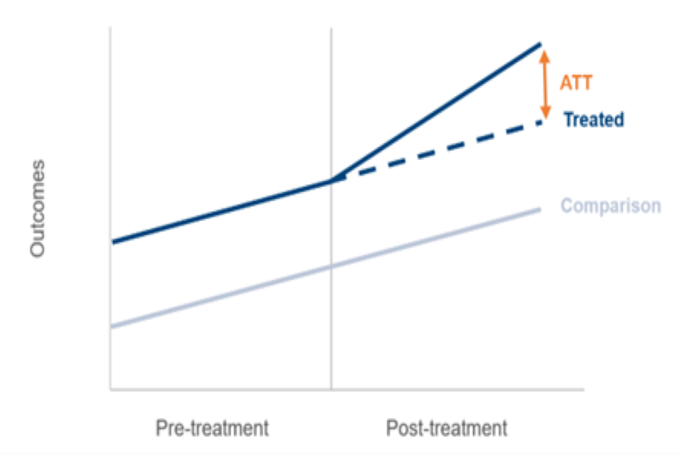
It is possible that the common trend assumption could be violated due to the voluntary nature of the ESF programme, causing the DiD estimator to fail. For example, individuals who participate on ESF may have higher levels of motivation, so may be more likely to experience positive employment outcomes resulting in different outcome paths, violating the assumption. However, we do control for several variables that proxy for motivation which should eliminate any bias this may introduce.

The impact charts presented in Section 3 are difference-in-difference adjusted impacts of the programme on each of the outcomes of interest.

2.3 Treatment and Comparison Groups

In this section we describe the characteristics of ESF participants and non-participants in the employment benefit, unemployment benefit and inactive benefit group. Table 3 lists summary statistics detailing personal / demographic characteristics and benefit receipt. This table includes only a few of the key characteristics. We note below some of the notable differences between participants and non-participants within each benefit group.

Table 3: Characteristics of the treatment group and (unmatched) comparison pool

	Employed Benefit	Employed Benefit	Unemployed Benefit	Unemployed Benefit	Inactive Benefit	Inactive Benefit
	Participants	Non-Participants	Participants	Non-Participants	Participants	Non-Participants
Observations	9,630	211,813	164,418	222,405	27,652	601,123

Personal / Demographic Characteristics

	Employed Benefit	Employed Benefit	Unemployed Benefit	Unemployed Benefit	Inactive Benefit	Inactive Benefit
	Participants	Non-Participants	Participants	Non-Participants	Participants	Non-Participants
Age (mean years)	34	35	36	36	36	43
Male (%)	52	50	64	58	53	45
Disabled (%)	18	15	31	24	45	40
Ethnic Minority (%)	15	12	22	14	12	9
Lone Parent (%)	15	13	11	10	12	12

Benefit Receipt

	Employed Benefit	Employed Benefit	Unemployed Benefit	Unemployed Benefit	Inactive Benefit	Inactive Benefit
	Participants	Non-Participants	Participants	Non-Participants	Participants	Non-Participants
Receiving UCE at ESF start (%)	100	100	0	0	0	0
Receiving JSA at ESF start (%)	0	0	41	20	0	0
Receiving UCU at ESF start (%)	0	0	59	80	0	0
Receiving ESA at ESF start (%)	0	0	0	0	69	65
Receiving UCI at ESF start (%)	0	0	0	0	31	35
Benefit Duration at start of Programme (mean weeks)	19	10	29	16	55	50

2.3.1 Employment benefit claimants: comparing ESF participants with non-participants

The mean age of an ESF participant in receipt of employment benefits is 34, compared with 35 for a non-participant. And there is a higher rate of disability among participants (18%) than non-participants (15%).

There is a higher proportion of ethnic minorities among participants (15%) than non-participants (12%). Similarly, a higher proportion of participants (15%) are lone parents compared to non-participants (13%).

All participants and non-participants (100%) are receiving UCE at the start of ESF, with participants on benefits for longer before the start of the programme – 19 weeks compared to 10 weeks.

Overall, these statistics suggest that employment benefit claimants who participate on ESF are slightly more disadvantaged than employment benefit claimants who do not participate. Our view is that these differences are not substantial and therefore the groups are largely similar.

2.3.1 Unemployment benefit claimants: comparing ESF participants with non-participants

The mean age of an ESF participants and non-participants in receipt of unemployment benefits is 36. A higher proportion of participants (64%) are male compared to non-participants (58%). There is also a higher rate of disability among participants (31%) than non-participants (24%).

There are more ethnic minorities among participants (22%) than non-participants (14%). And there are similar proportions of lone parents in both groups.

More participants are receiving JSA at the start of their ESF spell (41%) than non-participants (20%), with more non-participants in receipt of UCU at the start of ESF (80%) than participants (59%). Participants on average spent almost twice as long on benefits before starting the programme (29 weeks) than non-participants (16 weeks).

Overall, these statistics suggest that unemployment benefit claimants who participate on ESF are more disadvantaged than unemployment benefit claimants who do not participate.

2.3.1 Inactive benefit claimants: comparing ESF participants with non-participants

The mean age of an ESF participant in receipt of inactive benefits is lower at 36, compared with 43 for a non-participant. More than half of participants (53%) are male compared to less than half of non-participants (45%) who are male.

There is a higher rate of disability among participants (45%) than non-participants (40%). Similarly, a greater proportion of participants (10%) are ethnic minority compared to non-participants (8%). The proportion of lone parents among participants and non-participants is the same in both groups (12%).

The proportion in receipt of ESA at the start/pseudo start of ESF is slightly higher among participants (69%) compared to non-participants (65%), with the remainder receiving UCI (31% for participants and 35% for non-participants). Participants spent slightly longer on benefits (55 weeks) before starting the programme than non-participants (50 weeks).

Overall, these statistics suggest that inactive benefit claimants who participate on ESF are slightly more disadvantaged than inactive benefit claimants who do not participate.

2.4 Limitations

In this section we describe the limitations of the data and methodology we use to produce our analysis.

2.4.1 Data

Due to the design of the programme, we are unable to get participant National Insurance Numbers (NINos) through the management information (MI) data collection from projects. NINos are required to gather data on participants’ benefit and employment histories. This analysis uses a fuzzy match process – using the data we do have to match individuals to existing databases – to retrieve these. However, this process is only successful for around half (52%) of participants therefore, the treatment group consists of ESF participants we have a NINo match for. It may mean some people who participated in ESF are in the control group as we don’t have a NINo to identify them. We take a probabilistic approach to remove some people who we believe may be in this scenario but cannot be sure of complete removal. This may bias the results, but we cannot determine in which way.

The treatment group is further restricted to participants who are claiming benefits when they started ESF provision. This is because the PSM methodology we use requires us to have a substantial amount of data on individuals to successfully match up participants and non-participants. While we have sufficient data on ESF participants from the MI, we require the same for non-participants to find individuals for our comparison pool. Most data we have in DWP is related to DWP customers – primarily benefit claimants. For this reason, our analysis is focused on this group of people. However, just over one third (35%) of participants in the treatment group were claiming benefits when starting provision. Therefore, it must be taken into account that the results of the impact analysis may not represent all participants.

Figure 5 shows the final group of 2.35m participants, comprising the main analysis group used in the PSM, represented approximately 35% of the participants we have a NINo match for.

Figure 5: Diagram showing the numbers of participants and the stages at which they were excluded from the analysis.

2.4.2 Methodology

We chose to use propensity score matching (PSM) based on expert advice and because this approach was recommended in an externally commissioned feasibility report. However, the credibility of this approach depends on the ability to control for factors influencing an individual’s decision to participate in the programme, such as intrinsic ability, motivation, determination etc., as well as the outcomes they are likely to achieve as a result.

However, in practice it is not always possible to account for every factor that could influence participation because these may be unobserved in the data. For example, it is difficult to capture a participant’s motivation to join a programme. We assume that those choosing to participate on voluntary programmes like ESF may have a higher level of motivation to find employment than those who do not, and so may be more likely to achieve positive employment outcomes. Failing to account for these differences in attributes between the treatment and comparison groups could lead to the estimated impact being overstated^{[footnote 18]}.However, by including a rich history of labour market outcomes and benefit history, we attempt to overcome any biases in the results.

Chapter 3: Results

This section presents the results of the impact analysis for the European Social Fund (ESF) participants who started ESF after 2015, for the three-year period after they started the intervention. As discussed in Section 2.1, we have performed separate analysis for three main groups of participants:

1. Employed Benefits Group
2. Unemployed Benefits Group
3. Inactive Benefits Group

The outcomes of the PSM are set out in Section 3.1. The findings are set out in Section 3.2 with discussion of our understanding of the differing impacts in Section 3.3.

3.1 Outcomes of Propensity Score Matching

A preliminary check when assessing the quality of the matching process is to investigate the ‘common support’. This indicates what proportion of the treatment group observations have matched comparison group observations.

When we are unable to find a match within the calliper for a treatment group observation, these are dropped from the analysis. This is referred to as ‘off-support’. The more treated group observations that are dropped from this process, the less accurate the impact estimates are likely to be, reducing the representativeness of the results.

Table 4, 5 and 6 show the size of the treatment and comparison groups before and after matching, and the proportion of treatment with common support for the employed, unemployed and inactive groups.

Table 4: Size of treatment and comparison groups before and after matching and the proportion of treatment on support for the employed group

Sample	Size before matching	Size after matching	Proportion on support
Treatment	9,630	9,230	96%
Comparison	211,813	9,230	N/A

Table 5: Size of treatment and comparison groups before and after matching and the proportion of treatment on support for the unemployed group

Sample	Size before matching	Size after matching	Proportion on support
Treatment	164,418	163,060	99%
Comparison	222,405	163,060	N/A

Table 6: Size of treatment and comparison groups before and after matching and the proportion of treatment on support for the inactive group

Sample	Size before matching	Size after matching	Proportion on support
Treatment	27,652	27,285	99%
Comparison	596,849	27,285	N/A

The vast majority of the employed, unemployed and inactive benefit treatment groups were on support (96%, 99% and 99% respectively). This means that a match can be found for at least 96% of the observations in each treatment sample.

3.2 Findings from Impact Analysis

We present below our impact estimates of the ESF employment programme on our three main analysis groups: employed benefit claimants, unemployed benefit claimants and inactive benefit claimants.

All figures in this sub-section illustrate the impact in the two years prior to programme start, at the point of programme start and three years post programme start. The orange-coloured charts show the percentage of matched treatment and control groups in each category, i.e. percentage claiming benefits or in employment. The difference (or impact of the programme) is shown in the blue coloured charts. These charts show a 95% confidence interval (which is represented by the shaded area) around the central impact estimates (represented by the solid line).

3.2.1 Employment impacts

Figure 6 shows the impact of ESF provision had on the number of people in each benefit category with regards to their employment status over a three-year period following programme participation. An estimate of ESF’s impact is made by comparing the outcomes of participants against a comparison group who did not participate on the programme. The difference between the groups can be interpreted as an estimate of the impact of the programme.

The key result across all three benefit groups is that ESF participants are more likely to be in or remain in employment in the three years post programme start than had they not participated in the programme, and all of the differences are statistically significant.

Figure 6: Charts showing the employment outcomes and impacts of the programme – (a) outcomes and (b) impacts for the employed benefit group; (c) outcomes and (d) impacts for the unemployed benefit group; (e) outcomes and (f) impacts for the inactive benefit group

Employed Benefit Group

The outcome plot for employed benefit claimants (Figure 6(a)) illustrates the proportion of participants in this group who gained or remained in employment gradually decreased over the three-year tracking period.

Figure 6(b) shows that the impact of the programme on employment outcomes for the employed benefit group is positive in the three years following participation (roughly between a 1 and 5 percentage points impact over the 3 years). This suggests participation slightly increased an individual’s chances of being in employment over this period. Though this effect is not statistically significant until week 7.

Overall, employed benefit participants are likely to spend an additional 30 days in employment across the three years compared to employed benefit non- participants, when the percentage point impact is converted into days.

Unemployed Benefit Group

Figure 6(c) shows an increase in the proportion of participants claiming unemployed benefits who are moving into or remaining in employment in the three years following participation.

Figure 6(d) shows that the impact of the programme on employment outcomes for the unemployed benefit group is positive for most of the three-year tracking period (finding a steady state between 3 and 4 percentage points). This suggests participation slightly increased an individual’s chances of being in employment over this period. This effect is statistically significant beyond week 7 over the three-year period.

Overall, unemployed benefit participants are likely to spend an additional 35 days in employment across the three years compared to unemployed benefit non-participants.

Inactive Benefit Group

Figure 6(e) shows a gradual increase in the proportion of participants in receipt of inactive benefits moving into or remaining in employment. Although this proportion of participants at the end of the three-year tracking period is around the same as the proportion of participants two years prior to ESF start date.

Figure 6(f) shows that the impact of the programme on employment outcomes for the inactive benefit group is significantly positive in each of the three years following participation (reaching a steady state between 7 and 9 percentage points). This indicates participation substantially increased an individual’s chances of being in employment over this period. Beyond week 3, this effect is statistically significant over the three-year period.

Overall, inactive benefit participants are likely to be in employment for an additional 76 days across the three years than inactive benefit individuals who did not participate in an ESF programme. And those not in employment are moving towards “unemployment”, thus closer to the labour market.

3.2.2 Benefit impacts

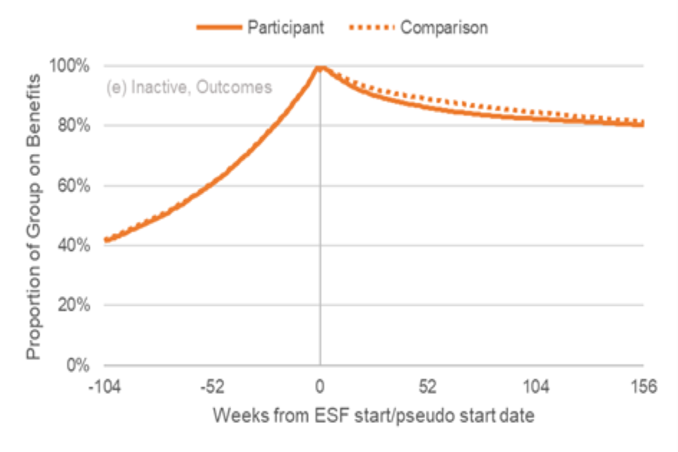
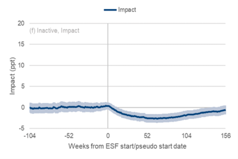
Figure 7 shows the impact of ESF provision on the number of people in each benefit category with regards to their benefit status over a three-year period following programme participation. The participants are compared to a comparison group used to estimate the outcomes had the participants not participated on an ESF programme. The difference between the groups can be interpreted as an estimate of the impact of the programme.

A key result here is we see the greatest impact of the programme on the inactive benefit group, which arguably are the hardest to help individuals within the labour market. This group spent more time in employment and less time on benefits over the three-year period as a result of programme participation, compared to the comparison group who did not participate.

Figure 7: Charts showing the benefit outcomes and impacts of the programme – (a) outcomes and (b) impacts for the employed benefit group; (c) outcomes and (d) impacts for the unemployed benefit group; (e) outcomes and (f) impacts for the inactive benefit group^{[footnote 19]}

Employed

Unemployed

Inactive

Impact on employed benefit receipt

The outcome plot for the employed benefit claimants (Figure 7(a)) illustrates the proportion of participants in this group who were in receipt of employed benefits decreases over the three-year tracking period since ESF start date for both participant and comparison groups.

Figure 7(b) shows that the impact of the programme on the proportion on employed benefits for this group is positive in the three-year following participation (reaching a steady state within the first year between 1 and 5 percentage points). This suggests participation slightly increased an individual’s chances of being on employed benefits over this period. Though this effect is not statistically significant until week 17.

Overall, employed benefit participants are estimated to spend an additional 27 days on employed benefits across the three years compared to employed benefit non-participants. However, as described in the employment impacts section, employed benefit participants are also more likely to be in employment following programme participation compared to those in the comparison group. Therefore, it is likely these participants are remaining in work although perhaps not earning enough to “flow off” Universal Credit.

Impact on unemployed benefit receipt

Figure 7(c) shows the proportion of participants in receipt of unemployed benefits who are remaining on unemployed benefits decreases over the three-year tracking period.

However, Figure 7(d) shows that the impact of the programme on benefit activity for the unemployed benefit group is largely positive for the three years following participation (it seems to still not have reached a steady state with it peaking between 15 and 16 percentage points). This suggests participation greatly increases an individual’s chances of being on unemployed benefits over this period. This effect is substantially statistically significant over the three-year period.

Overall, unemployed benefit participants are likely to spend an additional 140 days on unemployed benefits across the three-years compared to non-participants. But as described in the previous sub-section, unemployed benefit participants are also more likely to be in employment following participation, than unemployed benefit individuals who did not participate. Therefore, it is likely these participants are moving into employment with the support of Universal Credit.

Impact on inactive benefit receipt

Figure 7(e) shows a gradual decrease in the proportion of inactive benefit participants who are claiming inactive benefits over the three-year tracking period since ESF start.

Figure 7(f) shows that the impact of the programme on benefit activity for the inactive benefit group is negative in each of the three years following participation (reaching its lowest point between negative 2 and 4 percentage points). This indicates participation decreased an individual’s chances of being on inactive benefits over this period. Beyond week 136 this effect is not statistically significant.

Overall, inactive benefit participants are less likely to be claiming inactive benefits for an additional 20 days across the three years than inactive benefit individuals who did not participate on an ESF programme.

3.3 Understanding from Differing Impacts

It is evident from the impact estimates in the previous section that the effects of the ESF programme vary across the benefit groups. With the greatest impact being on the inactive benefit claimants, given this group spent more time in employment and less time on benefits over the three-year period as a result of programme participation, compared to the comparison group who did not participate.

In this section, we discuss some possible explanations for the observed impacts of ESF provision on participants in receipt of employed, unemployed and inactive benefits.

Voluntary programme

As ESF is a voluntary programme, it is possible that those who choose to take up provision are more motivated than those who do not take-up support. Therefore, for active benefit claimants this might translate into better work-search habits and for the inactive group a greater willingness to engage. This could lead to differing results between the groups.

Programme ‘lock in’ effect

Participants receiving employment programme support often don’t flow off benefit in the early part, as they are engaged in the support that the programme offers them as most provision lasts several months. Therefore, they may continue to claim benefits to access the support whereas without ESF, they may have simply stopped. Equally, they may undertake formal or informal training in preparation for taking up employment at a later date.

This can often cause a delay in participants transitioning away from benefits, which may help explain the small “dip” in impact as seen for the employed and unemployed benefit recipients. It may also explain the sharp initial net rise in the impact on benefit receipt following the start of ESF provision. Some of these findings are corroborated by the survey responses which cannot be compared in the counterfactual.

Unobserved programme benefits

The programme has been successful in bringing participants closer to the labour market, although not always to the extent where they secure employment or cease receiving benefits. However, the programme has yielded softer outcomes such as enhanced skills, confidence and motivation, which are reported as positive outcomes in the MI but are not currently captured in the impact measures. These softer outcomes may lead participants to have higher expectations for jobs, causing them to reject less desirable job offers, thus prolonging their job search – which again is not currently accounted for in our analysis but are evidenced in other ESF evaluations for example The Leavers Survey^{[footnote 20]}, where participants reported increases in softer outcomes. Although, we cannot compare these with a counterfactual.

Chapter 4: Cost Benefit Analysis

This section presents a Social Cost Benefit Analysis (SCBA) of European Social Fund for participants who started ESF on benefit after 2015, for the three-year period after they started the intervention.

The methodology is set out in section 4.1. The findings are set out in 4.2 with a form of sensitivity analysis in section 4.3 and conclusions in 4.4.

4.1 Social Cost Benefit Analysis methodology

The methodology underpinning the CBA of ESF is based on the Department for Work and Pensions (DWP) Social Cost Benefit Analysis framework, as set out in Working Paper 86^{[footnote 21]}.

4.1.1 Estimating additional days in employment

The impacts in section 3 show the percentage point impact of moving people into employment, at 36 months. However, for the SCBA we are only concerned with the number of additional days in employment to calculate the financial benefits from this outcome.

To calculate this, the sub-group impacts were aggregated up to produce an overall estimate of impact for the whole treatment group. This was then transformed into an “additional days” figure. This gave the impact that over the 36-month period following start on ESF, individuals spent on average an additional 39.7 days in employment.

People who are on inactive benefits when they start ESF, on average, have the greater employment impact with around 76 days of additional employment compared to those that do not participate in ESF. For those who start ESF unemployed the impact is around 34 days compared to the comparison group, and for those who start ESF already employed the impact is around 30 days.

4.1.2 Perspectives under consideration

The SCBA will consider two key perspectives when calculating the costs and benefits of ESF, these are:

• the Exchequer, i.e. the government financial perspective
• society

The exchequer perspective is quite a narrow focus as it only considers the direct fiscal elements of the policy that affect government. As a result, this perspective focuses on the tax and fiscal spending, including income and indirect taxes, National Insurance and social security expenditure. The social perspective considers a much broader range of outputs which fits with the focus on ESF being on wider elements than just the labour market. The social element includes things such as output from employment (i.e., the value of goods/services produced), travel costs to employment, childcare and healthcare benefits.

For the purposes of the analysis “society” refers to the aggregate of British citizens. Therefore, a cost or benefit to participants, their employers or the exchequer can also represent a cost or benefit to society. However, in practice a number of these gross impacts are essentially “transfer payments”. These represent a cost to one party but a benefit to another, and therefore offset. For example, the wages earned by an individual are a benefit to them but a cost to their employer and therefore these offset.

Once the costs and benefits have been calculated a Cost Benefit Ratio (CBR) can be produced show the relative balance of the two. If the total is greater than £1 then for every pound spent on ESF then there is a positive ratio, or to put another way a ratio of £1:£1 is break-even.

4.1.3 Calculating benefits

In our calculations around benefits a number of assumptions are made, for example the composition of the target group and wage rates, these are set out in Annex 7.

Increase in Output

This specifically refers to the economic output produced by ESF participants in the additional days they spend in employment. This output represents a benefit to employers, who then sell the output, and to society, who consume it. In the impact analysis we do not attempt to measure the value of this output, and therefore make several assumptions to produce it.

It is assumed that the labour market is perfectly competitive, therefore that employers will hire workers only up to the point where their additional unit of output is equal to their associated marginal cost. The cost of production, and therefore the value of the output produced during the additional days in employment, is assumed to be equal the gross wage payments and employers’ National Insurance contributions.

Reduction in operational costs

ESF participants will, on average, get less support from Jobcentre Work Coaches in the three years post-start as they are more likely to be in employment, and therefore less likely to be in the intensive support regimes that require the most intensive Work Coach time. It also means that ESF participants are less likely to go on other employment programmes, which cost resource. This translates to operational savings which represent a benefit to society and the Exchequer, as resources can be allocated to other alternatives.  

Change in time spent in benefits

As a result, of time spent on ESF, participants are more likely to be in employment. Under UC this makes for a complex picture, ESF participants spend more time on benefits overall, but less time on inactive benefits as well as the employment impact. This implies that the amount of benefit received overall could be lower, as active benefit rates tend to be lower and UC would provide a “top up” to earnings. This impact analysis does not quantify the change in earnings to allow us to verify this, so it is necessary to make assumptions in this space.

The reduction in benefits represents a benefit to the Exchequer, but no net cost or benefit to society, except via redistributive effects explained below.

Increases in taxes

This pertains to the increase in income tax, National Insurance contributions and indirect tax (for example, VAT) that accrues when an individual moves into employment because of time on ESF. This represents a benefit to the Exchequer but no net cost or benefit to society as a whole, except via redistributive effects explained below.

Increase in travel costs

As a result of people moving into additional time in employment additional travel and childcare costs also accrue. These represent a cost to society as the provision of travel and childcare services diverts resources from other uses.

In the SCBA model we cap the number of times money can circulate around the economy for simplicity. In this example travel costs could generate income for firms such as transport companies and childminders, but these are not included in our SCBA framework.

Reduction in healthcare costs

Evidence has shown that people who move into employment are less likely to make demands on the National Health Service (NHS), via lower Accident and Emergency admissions. The evidence found that the link is causal and that moving into employment is a driver. Therefore, there is a saving to the Exchequer as a result of reductions in NHS expenditure, and society, as economic resources can be allocated to other purposes either within the NHS or elsewhere.

Redistributive costs and benefits

This refers to the redistributive costs and benefits associated with monetary transfers between participants, employers and the Exchequer. In line with the methodology prescribed in the HM Treasury Green Book^{[footnote 22]}, participants, who have relatively low incomes, are assumed to value each additional pound more highly than employers and the average taxpayer, who both have a relatively high income compared to participants. This implies, for example, that monetary transfers from the Exchequer to participants represent a benefit to society as a whole. In line with the recommendations of Fujiwara (2010), redistributive costs and benefits are estimated by applying a ‘welfare weight’ of 2.4 to monetary transfers made to and from programme participants.

4.1.4 Calculating costs

Calculating the CBR uses a flat unit cost, that is aggregated across all participants. It is a negative exchequer and societal impact by default.

The unit cost was calculated specific to the participants in the treatment group. When conducting the analysis, we identified the projects each participant in the sample was from, then used the current unit cost for that project.

For example, if 100 of the ESF participants in the treatment group were from Project A at a unit cost of £2000 per participant and another 150 were from project B at a cost of £2500 per participant, and so on. To calculate the unit cost we multiplied 1002000 and 1502500 to give a total cost of £575,000 (in this simplified example) and then divided by 250 to give a unit cost of £2,300 (again, only in this example).

As we are only interested in the additional unit cost of ESF, we do not need to make a similar calculation for the control group.

4.2 Social Cost Benefit Analysis findings

Table 7 below shows the breakdown of the CBA findings from both the exchequer and social perspectives, at the 36-month post-start point.

(Figures rounded to nearest £5)	Perspective
ESF impacts	Exchequer	Society
Increase in Output	-	£2,350
Operational Costs	£20	£20
Reduction in benefits	£900	-
Increase in taxes	£570	-
Increase in travel costs	-	-£35
Reduction in healthcare costs	£90	£90
Redistributive costs & benefits	-	£1,040
Total Costs	-£2,300	-£2,300
Net Benefit	-£720	£1,160
Cost Benefit Ratio	£0.69	£1.50

At the three-year point, the CBR is below £1 for the exchequer but above £1 for the social. The exchequer perspective is fairly narrow in scope, particularly for a programme like ESF. It only considers the direct impact of taxes and benefits from the employment element of the programme and won’t consider wider impacts, such as additional output. Neither the exchequer, nor the social, benefits include the impacts of more education, reductions in crime or negative behaviour. At the three year point the benefits that are observed and monetised here are not sufficient to outweigh the unit cost, leading to a net loss of £720 and a CBR of £0.69.

The social benefit is greater than the cost of the programme at the three-year point. Factoring in output and the welfare weight of moving these individuals into work generates a £1,160 surplus to society. The societal perspective considers the redistributive benefits generated from the marginal pound, as it is worth relatively more to the participants of ESF – who are likely to be, overall, from the lower earnings quintiles pre-ESF compared to the average taxpayer. The CBR is £1.50, meaning a 50p “surplus” for every pound spent on ESF.

Table 8 shows the cost benefit ratios at year 1, 2 and 3 of tracking. As time progresses the more outcomes accrue. Several studies have indicated that the longer tracking periods available the more benefits increase. In our analysis, even after three years the impact has not trended back to zero this suggests that the impacts continue past the three-year point with additional days in employment still being seen in years 4+ following start. The costs are, effectively, fixed as they accrue when the participants start on an ESF project therefore, any more outcomes serve to increase the benefits and therefore the CBR.

Table 8: Cost benefit ratios over time

Tracking period	Exchequer	Social
12 months	£0.16	£0.35
24 months	£0.43	£0.93
36 months	£0.69	£1.50

The 12-month point has relatively low CBR. This is to be expected as the period is 12-months post-start, so the majority of people will likely still be receiving ESF support – and the ones who are not and achieved outcomes are more likely to be “deadweight”. After 24-months the CBRs increase dramatically, as more people see the impact of ESF and start to gain more outcomes. Some people may still be on ESF but are gaining outcomes at a higher rate than those that did not start. This trend continues into the 36-month point. Even here, as stated above, the difference between the treatment and non-treatments groups is not zero suggesting that more additional outcomes could be achieved if we had the data to track 48- or 60-months post-start.

4.3 Social Cost Benefit Analysis of differing groups and sensitivity analysis

The analysis has centred on the whole of the group of people who are on benefit upon starting ESF. However, unlike other labour market programmes the characteristics of participants is varied. Even just looking at the conditionality regimes they are part of whilst being on benefit demonstrates this fact.

Programmes like Restart and Kickstart, the vast majority of participants are on Universal Credit and in the Intensive Work Search (IWS) regime. Therefore, they are all on a singular benefit and unemployed. However, for ESF those on benefits upon starting includes those that started pre-UC and may have been on Jobseekers’ Allowance (JSA), Employment and Support Allowance (ESA) or many other benefits. Even those who were on UC are not all drawn from the IWS regime.

Rather than splitting the analysis by the many types of benefits, we have produced impacts that show the variation between types of conditionality. Specifically, how it varies between those that are unemployed, those who are inactive and those who are employed when they start on ESF. Those who are employed, also must be on benefits which limits the sample.

We take this approach to show an element of sensitivity to our central estimate, as it shows the range of potential CBR if other impacts were observed. This also shows that sensitivity without creating spurious scenarios that would not likely occur. We also show the different estimates for different tracking periods to further develop the range of potential CBRs.

Overall, the group in the main analysis is made up of around 4% of people who were employed upon start, around 19% who were inactive and 77% who were unemployed. So, whilst unemployed makes up the largest group, nearly ¼ of the sample were not unemployed.

The results are different across these groups, as you may expect. Table 9 below shows the various CBRs of these three groups, at the 36-month point.

Table 9: Cost benefit ratios, at 36-month point for different groups

	CBR	CBR
Group	Exchequer	Social
Employed	£0.55	£1.23
Inactive	£1.17	£2.68
Unemployed	£0.60	£1.30

The results are the greatest for the inactive group. The impacts are higher for this group, which is in keeping with the core purpose of ESF interventions as they aim to help those who are furthest away from the labour market. The results for unemployed are the next and employed lowest.

Conclusions should not be drawn as to whether ESF is more effective at helping one group versus another, as there are several factors that may influence the difference between the types of participant. For example, for the employed group “additional days in employment” may be the wrong way to measure impact and a better way may be earnings – data limitations have prevented this approach being undertaken, at this stage.  Similarly, the 36 months may not be a sufficiently long tracking period for the unemployed (for example) to see the same impacts as the inactive.

As with the core analysis it is possible to use the 12-, 24- and 36-month tracking periods to show further ways the CBRs breakdown. Table 10 shows these various breakdowns of each of the group, using each of the tracking periods.

Table 10: CBRs for each group, in each tracking period.

	CBR	CBR
12 months	Exchequer	Social
Employed	£0.17	£0.37
Inactive	£0.27	£0.62
Unemployed	£0.14	£0.30

	CBR	CBR
24 months	Exchequer	Social
Employed	£0.37	£0.82
Inactive	£0.72	£1.63
Unemployed	£0.38	£0.81

	CBR	CBR
36 months	Exchequer	Social
Employed	£0.55	£1.23
Inactive	£1.17	£2.68
Unemployed	£0.60	£1.30

In each instance, the patterns are the same as the overall and the group-based trends. Inactive people on ESF have the greater CBR. Unemployed starts to deviate from employed after year one but remains behind inactive. The three do not follow the exact same pattern, which demonstrates that the different groups see outcomes at different times, which is expected.

As before, we urge caution in reading too much into these differences. The characteristics are different between the groups as, likely are the outcomes. They are presented as a means of sensitivity analysis for the CBA and purely for illustration.

We have also used the 95% confidence intervals on additional days in employment, to produce some upper and lower bound estimates for the CBR as shown in Table 11.

Table 11: CBR for each group at either side of the Confidence Intervals

	Lower bound- CBR	Lower bound- CBR	Upper Bound- CBR	Upper Bound- CBR
12 months	Exchequer	Social	Exchequer	Social
Employed	£0.03	£0.07	£0.31	£0.68
Inactive	£0.21	£0.47	£0.33	£0.76
Unemployed	£0.11	£0.23	£0.17	£0.37

	Lower bound- CBR	Lower bound- CBR	Upper Bound- CBR	Upper Bound- CBR
24 months	Exchequer	Social	Exchequer	Social
Employed	£0.09	£0.21	£0.64	£1.43
Inactive	£0.59	£1.34	£0.84	£1.92
Unemployed	£0.32	£0.68	£0.44	£0.94

	Lower bound- CBR	Lower bound- CBR	Upper Bound- CBR	Upper Bound- CBR
36 months	Exchequer	Social	Exchequer	Social
Employed	£0.14	£0.32	£0.96	£2.16
Inactive	£0.98	£2.24	£1.36	£3.11
Unemployed	£0.51	£1.10	£0.69	£1.50

From this we can see that there is some sensitivity in the SCBA estimates that come from differing impacts. However, the range does not significant alter the overall conclusion about the success, or otherwise, of ESF.

Some further sensitivity analysis was undertaken on the assumptions set out in Appendix 7. This is not presented in the report as the range of potential values is substantial but would need evidencing to include as a central case. For example, not using NLW would have a potentially significant impact on the SCBA figures as the model is highly sensitive to earnings impacts. However, no evidence supports the use of an alternative figure, as a result would likely require further assumptions to justify.

4.4 Cost Benefit Analysis conclusion

The Cost Benefit figures show a positive return on expenditure on the societal perspective, but lower return on exchequer. Given that the maximum amount of time on ESF is three years, it might be that three years after an individual starts on ESF may not be sufficient time to receive the intervention and gain employment. These individuals may have achieved intermediate outcomes, but not yet employment particularly if they were significantly hard to help.

Many ESF participants faces multiple disadvantages, and for much of ESF provision having additional “barriers”, is a pre-requisite for being on the programme. In general, harder to help individuals do not generate significant returns particularly on the exchequer perspective, and if we only track outcomes for a small number of years. This is common across many labour market programmes. It could be the time horizon as previously mentioned or may be because the unit costs required to help those who have more barriers are relatively high and would need longer periods in employment to produce a positive return on investment.

Another factor is that for some of these individuals they will achieve other outcomes that are not monetised. For example, alcohol and drug issues are relatively common across some ESF participants yet we do not account for the health or crime savings from dealing with these issues as part of the CBA.

Furthermore, as stated previously a significant proportion of ESF participants are in employment upon starting. Roughly 1/3 of all expenditure is on people that are not inactive or unemployed upon starting. We would not expect the impacts of ESF to be on additional time in employment, or off benefits, but in higher wages and progression which these figures do not measure.

This is not an exhaustive list. However, it should be noted that despite all those caveats the CBRs are encouraging. The societal benefit is greater than £1 across all groups at the 36-month point and across all participants from the 24-month point onwards. The increase in the exchequer benefits suggest that the programme would generate enough exchequer benefits – on this relatively narrow definition of just DWP exchequer benefits – for all groups once a 48-month tracking period has been observed. It is also the case that it does at the 36-month point for the harder to help groups within this analysis. These are all positive outcomes from this work.

Chapter 5: Conclusions

5.1 Impact Analysis

The analysis uses an average treatment effect on the treated (ATT) to estimate the impact of ESF on participants. It uses a Propensity Score Matching (PSM) approach to compare the outcomes of those who went on ESF with those of a similar group who did not. Both groups were on benefits at the point of starting, in the case of participants, and pseudo-start, in the case of those that are not participants.

PSM approaches use a large amount of data on participant characteristics to control for various demographic traits that potentially influence labour market outcomes outside of ESF. The aim of the approach is to estimate the direct impact of the ESF programme.

The analysis splits participants into groups based on the type of benefits they are claiming on starting, whether they are unemployed, employed or inactive. This helps to account for the likely differences in labour market regime that occurs between groups.

The data used allows us to measure the number of additional days in employment that accrue at the three-year point, post start on ESF. For the control group this is measured by assigning the pseudo-start date, based on a distribution of their benefit start dates. This is the basis of the central estimate.

Our central case produces an estimate on the amount of additional time spent on active benefits, inactive benefits and employment. The primary outcome, however, is employment – which we use for the Cost Benefit Analysis (CBA). Whilst there is variation by benefit type upon starting, the central figure is that ESF participants spend around 40 days more in employment than similar non-participants.

A significant amount of sensitivity analysis has been carried out to ensure these estimates are robust as possible. In conjunction with the academics named at the start of the report we have altered the regression running both a probit and logit approach, changed the callipers and other technical elements that are not presented in this report. We have also shown the potential range of outcomes in the form of the confidence intervals that we do include.  Also presented in this analysis are estimates that show the various impacts on different types of outcomes, subset by the different benefit groups upon starting. Each show that the treatment group has a similar outcome over and above the comparison group. The results show the ESF is more likely to move inactive participants away from inactive benefits and subsequently into employment.

The ESF programme is voluntary. Whilst we do control for lots of observed characteristics and attempt to do so for unobserved, there could be further factors like motivation that may have the effect of creating bias in the results. However, there are also several outcomes that we know providers deliver which are not estimated in this analysis which may offset this.

ESF begins to deliver impacts within the first year, despite some people still being on the programme at that point. Outcomes build over time for all participants, in each of the main analysis groups. People start to move into employment and, for those that don’t, many move onto “active” benefits which, in the longer term, should mean they are more likely to gain employment in the future.

5.2 Cost Benefit Analysis

Using the impact analysis results, a Cost Benefit Analysis was undertaken to show the cost effectiveness of ESF over time. Primarily this was done at three years, but also at one and two years.

The analysis looks at the cost effectiveness from the exchequer and societal perspectives, as each value costs and benefits in a slightly different way. At the three-year point, for every pound invested:

• The exchequer benefits by £0.69
• Society benefits by £1.50

Sensitivity analysis on the Exchequer and society perspectives show that these results are consistent across various assumptions. The exchequer costs include all wages paid to participants, whereas society only includes these as a transfer payment. This is a large portion of the cost, so this discrepancy leads to a significant difference in results between these perspectives.

If we look at subgroups, for every pound invested:

Those who are employed on starting

• £0.55 in exchequer benefits
• £1.23 in society benefits

Those who are unemployed on starting

• £0.60 in exchequer benefits
• £1.30 in society benefits

Those who are inactive on starting

• £1.17 in exchequer benefits
• £2.68 in society benefits

It is worth observing that even at the three-year point, the impact estimate graphs are not zero. This means that even after three years, whilst there is some expected decay, the positive results are on-going. This would give us reasonable confidence that the impacts of ESF carry on after three years. Given that the costs would be fixed, any further additional time in employment would generate more benefits at the same cost and therefore improve the cost benefit ratios.

It is also the case that whilst not exactly alike, these results are broadly in line with the YEI impact estimates and CBA figures, from the published report.^{[footnote 23]} The main difference being that impacts were only tracked for 12 months, compared to 36 therefore not as many will have accrued, potentially limiting the amount of benefit observed.

It is important to reiterate that the accuracy of any cost and benefit estimates is very much dependent on the robustness of the impact estimates from which they are derived and the validity of the assumptions upon which they are based. It should also be borne in mind that a number of potentially significant costs and benefits have been excluded from this analysis due to a lack of either data or a robust method existing within DWP. These include impacts on crime, health (outside of narrow NHS costs), alcohol and drug abuse as well as things like increased motivation.

These results are consistent with the wider ESF evidence base. Overall, participants have benefitted by getting outcomes at a relatively high rate. For many this has come from a low base, as they have required multiple barriers to be addressed before they can achieve some of the cashable outcomes measurable in the CBA. Qualitative research on ESF has shown that its most successful in providing wraparound support for these hardest to help individuals, which is often more costly, but potentially has some of the greatest longer-term payback.

Appendices

Appendix 1: Data sources

Data for the European Social Fund (ESF) was collected throughout the programme. This programme data (MI) includes identifiable information about participants and the date they started the programme, as well as general information about the programme. Participant contact data was also collected to enable us to match ESF data to DWP administrative data.

A wider set of characteristics are collected using administrative data. This allows for a much larger sample size (close to the population), allows variables and outcomes to be tracked over a long period.

We use administrative data from DWP, particularly from Universal Credit (UC) datasets and the National Benefits Database (NBD) for legacy benefits. These provide details of spells on DWP benefits, characteristics of DWP customers and spells on employment programmes including ESF. This is used to build up a detailed picture of an individual’s benefit history over time, which is then used in the matching.

We also use administrative data from His Majesties Revenue and Customs (HMRC) Tax System. This gives is detailed employment histories of claims and outcome measures to enable us to assess employment effects.

We combine all this information to construct an evaluation dataset containing the relevant variables for each claimant.

Appendix 2: Pseudo start dates

The European Social Fund (ESF) involved participants starting programmes at different times over several years. The benefit and employment outcomes of individual participants in our treatment group are measured weekly from the date on which they start provision. However, those in our comparison group have no natural start date from which outcomes can be measured. Therefore, it is necessary to assign a ‘pseudo-start date’ to all individuals in the control group that can be used in place of the intervention start dates.

We must ensure that these pseudo-start dates identify a period of time over which non-participants can best represent what would have happened to ESF participants had they not participated in the programme. The method we used for assigning the pseudo-start dates was to take the real start dates of the ESF participants and randomly assign them to the comparison group. These dates are assigned based on the distribution of start dates in the treatment group and the distribution of the lengths of time individuals in the treatment group had spent on benefits prior to starting provision. So within each start month (i.e. the month the individual started on the programme) the start date distributions of the comparison and treatment groups match up.

Appendix 3: Propensity Score Matching

For each participant and non-participant in the sample we compute a ‘propensity score’. This defines the probability of an individual participating on the ESF programme given their observed characteristics. We use a non-linear regression model – probit to calculate the scores, where participation is the dependent variable, and the observed characteristics are the independent variables. A full list of the variables we use in the propensity score matching is provided in Appendix 6.

After estimating the propensity score for each observation in our samples, we match each individual in the treatment group with individuals from the comparison group based on their propensity scores. We match individuals in the treatment group to many individuals in the comparison group, and the outcome of the treatment group is then controlled to the average of the matched individuals in the comparison group – this is referred to as Kernel ‘one-to-many’ matching.

For PSM to be a viable methodology, there must be sufficient common support for participants among the non-participant sample. This means we need to observe participants and non-participants with the same characteristics, so that we are effectively comparing only comparable individuals. To implement this common support, we use a bandwidth in the Kernel matching. This determines how closely the propensity score of a non-participant must be to that of a participant for selection into the final matched comparison group.

All non-participants in the sample with propensity scores within the Kernel bandwidth are selected and weighted using an Epanechnikov distribution. The bandwidth we use for our analysis is 0.0001 which although is much smaller than the standard bandwidth (0.06), it results in smaller bias and ensures a tighter match between participants and non-participants.

As part of the PSM process, each individual receives a weight. The weight assigned to non-participants depends on how many participants the non-participants match to, and how many other non-participants match to that participant. This essentially indicates their significance in the matching so that the number of weighted matched non-participant observations is equal to the number of matched participant observations.

The matching was carried out using an adaptation of the SBWA Evaluation Stata code in 2016, which relies on the Stata module psmatch2 written by Leuven and Sianesi (2003)^{[footnote 24]}. The matched-weighted sample is then used to check the quality of the matching and to estimate the impact (see Appendix 5).

Appendix 4: Non-participant samples

In preparation for carrying out matching methods, it is necessary to define a population of non-participants, known as a comparison pool, from which the final matched control group will be selected for comparison against the treatment group. To provide a suitable comparison pool of benefit claimants who did not participate on the ESF programme, we draw samples of non-participants mirroring as closely as possible the selection criteria used to draw the participant sample.

To compare outcomes of participants and non-participants at a time period such that non-participants can represent what would have happened to ESF participants if they had not participated, we randomly assign a pseudo start date to each non-participant in a way that matches the distribution of participant start dates. The pseudo start date for non-participants is treated as equivalent to the actual start date for participants. More details of how these dates are generated are provided in Appendix 2.

For inclusion in our analysis, individuals in the comparison pool must meet the following conditions:

• Those aged 19-64, in order to track some benefit history before pseudo start date
• Those who have a pseudo start date on or before September 2020 in order to track impacts for 3 years after pseudo start date
• Those who were claiming benefits at their pseudo start date, in order to have a sufficient amount of data for the matching methodology we use

Similarly to the treatment group, the comparison pool is split into three groups based on benefit type (see Table 1 for groupings).

The resulting comparison sample size is 1,035,341 participants. This is comprised of 211,813 employed benefit claimants, 222,405 unemployed benefit claimants and 601,123 inactive participants. It is important we have large comparison pools as this increases our chances of finding good matches.

Appendix 5: Outcomes of matching

To assess the success of the matching for our analytical run, we use the Rubin’s B and Rubin’s R and the maximum and median percent biases. Table 12 shows these results for the employed, unemployed and inactive groups.

Table 12: PSM summary statistics used to assess the success of the matching for the main analytical run

Benefit Group	Rubin’s B	Rubin’s R	Max % bias	Median % bias
Employed	7.93	1.49	2.32	0.28
Unemployed	14.3	0.92	6.36	0.43
Inactive	5.51	0.91	3.25	0.17

All of the metrics in the table above fall within the commonly accepted thresholds for the selected approach. For example, we would want the max bias to be below 5 and if this isn’t satisfied, we would check if the Rubin’s B statistic is less than 25 and the Rubin’s R statistic is between 0.5 and 2 for all benefit groups. This suggests matching has been successful in creating balanced treatment and comparison groups and they are comparable across the covariates used in the PSM.

Appendix 6: Description of Variables

We outline below in Table 13 the variables used in the analysis.

Table 13: Variables and values used in the analysis

Variable	Type	Values
Gender	Categorical	Male; Female
Age, (and Age squared)	Numerical	Integer values
Disability	Categorical	Not disabled; Disabled; Unknown
Ethnicity	Categorial	White, Black, Asian, Mixed, Chinese, Other, Unknown
Sought occupation	Categorical	26 broad categories: for example “Administrative”, “Health Professionals”, “Sales Occupations”
Lone Parent	Categorical	Lone Parent; Couple; Not a Parent; Unknown
Low Qualified	Categorical	No; Yes; Unknown
Refugee	Categorical	No; Yes; Unknown
Benefit start month	Categorical	126 months from March 2012 to September 2023
ESF start month	Categorical	66 months from March 2015 to September 2020
Benefit labour market history	Categorical	104 binary variables per benefit type – one representing each of the 104 weeks prior to ESF start date. Benefit types include: JSA, UCE, UCU, UCI, ESA. Values are: receiving benefit; not receiving benefit
Work labour market history	Categorical	104 binary variables – one representing each of the 104 weeks prior to ESF start date. Values are: in work; not in work
Benefit spell duration	Numerical	Integer values
Employment programme history	Categorical	19 binary variables – one representing participation in a different employment programme prior to ESF start date. Values are: on programme; not on programme

Appendix 7: Assumptions for benefits calculation

The impact analysis focused on estimating the additional time on, or off, benefits and in employment as a result of ESF. It did not attempt to estimate anything around additional earnings, number of hours worked, or amount of benefit received. Therefore, it is necessary to make a number of assumptions for use in the DWP Social Cost Benefit Analysis (SCBA) model.

The analysis uses ESF participant data to establish the proportion who were subject to a health journey, the proportions in different age groups (shown in section 2) as well characteristics around number of children and regions.

For other data, the analysis assumes that all participants moving into employment are earning the NLW in 2023/24 (£10.42 per hour, when this analysis was carried out), that they were working 37 hours a week and that housing costs were in line with UK average rental costs in 2023. It is also assumed where a participant had a child, that there is only one child, and the child is over 14. Indicative analysis suggests these are broadly sensible assumptions to make but equally, they are safe assumptions that should not bias the SCBA estimates too much. For example, assuming that participants had 2 children under 14 could add around 4% to the benefit figures in each instance.

1. DWP/Ecorys (2018), European Social Fund impact evaluation: research design and scoping study ↩

2. DWP (2013), The DWP Social Cost-Benefit Analysis framework (WP86) ↩

3. Available at: DWP research reports ↩

4. DWP Social Cost-Benefit Analysis framework. DWP Working Paper 86, 2010 (Fujiwara) ↩

5. See glossary for definition of ‘Inactive Benefit’ and ‘Active Benefit’ ↩

6. Dr Salis and Dr Speckesser were initially commissioned to advise on this project while working for the National Institute of Economic and Social Research through a DWP research contract with IFF Research.   ↩

7. See DWP Research series at: DWP research reports ↩

8. See glossary for definition of ‘pseudo-start’ ↩

9. Youth Employment Initiative: Process Evaluation (2017)  ↩

10. European Social Fund impact evaluation: research design and scoping study (2018)  ↩

11.  Early Impacts of the European Social Fund 2007 to 2013 (2011) ↩

12. European Social Fund and Youth Employment Initiative Leavers Survey Report 2016-2019 (2022)  ↩

13. Evaluation of the European Social Fund 2014-2020 Programme in England: Qualitative case study research (2022)  ↩

14. Youth Employment Initiative: Impact Evaluation (2022) ↩

15. At: Building Better Opportunities ↩

16. ESF 2007 to 2013: evaluation of the second half of the programme ↩

17. While we aimed to show impact at Priority Axis (PA) level, the employment status acts as a broad proxy. For example PA1 covers unemployed and inactive and PA2 covers employed. ↩

18. DWP Employment Data Lab ↩

19. See glossary for specifics about which benefits are considered in each group ↩

20. European Social Fund and Youth Employment Initiative Leavers Survey Report 2016-2019 (2022)  ↩

21. DWP SCBA framework, Working Paper 86 (2010), Fujiwara ↩

22. The Green Book (2022) - GOV.UK (www.gov.uk) ↩

23. DWP (2022), Youth Employment Initiative Impact Evaluation ↩

24. Leuven, E and Sianesi, B. (2003), psmatch2: Stata module to perform full Mahalanobis and propensity score matching, common support graphing, and covariate imbalance testing. ↩