Estimating Scottish taxpayer behaviour in response to Scottish Income Tax changes introduced in 2018 to 2019
Published 16 December 2021

© Crown copyright 2021
This publication is licensed under the terms of the Open Government Licence v3.0 except where otherwise stated. To view this licence, visit nationalarchives.gov.uk/doc/open-government-licence/version/3 or write to the Information Policy Team, The National Archives, Kew, London TW9 4DU, or email: psi@nationalarchives.gov.uk.
Where we have identified any third party copyright information you will need to obtain permission from the copyright holders concerned.
This publication is available at https://www.gov.uk/government/publications/estimating-scottish-taxpayer-behaviour-in-response-to-scottish-income-tax-changes-introduced-in-2018-to-2019/estimating-scottish-taxpayer-behaviour-in-response-to-scottish-income-tax-changes-introduced-in-2018-to-2019
1. Executive Summary
1.1 Background to Scottish Income Tax
- Income Tax has been partially devolved to the Scottish Parliament since tax year 2016 to 2017
- From tax year 2017 to 2018 it has had the power to set the rates and thresholds for the non-savings and non-dividends (NSND) Income Tax paid by Scottish taxpayers (often known as earned income)
- For the tax year 2018 to 2019, the Scottish Government introduced two new Income Tax bands and rates, as well as increasing the rates for two of the existing bands
- This switched Scotland from a three-band system to a five-band system - the tables below set out the rates and thresholds for Scottish Income Tax and for Income Tax in the rest of the UK (rUK)
Table 1: Scottish Income Tax NSND policy for the tax year 2018 to 2019.
| Tax band | Scottish threshold | Scottish Income Tax marginal rate |
|---|---|---|
| Starter rate | £11,850 | 19% |
| Basic rate | £13,850 | 20% |
| Intermediate rate | £24,000 | 21% |
| Higher rate | £43,430 | 41% |
| Top rate | £150,000 | 46% |
Table 2: rUK NSND Income Tax policy for the tax year 2018 to 2019.
| Tax band | rUK threshold | rUK marginal rate |
|---|---|---|
| Basic rate | £11,850 | 20% |
| Higher rate | £46,350 | 40% |
| Additional rate | £150,000 | 45% |
1.2 Aim of the study and the approach taken
- The changes to Scottish Income Tax provided a unique opportunity to better understand Scottish taxpayer behaviour in response to Income Tax changes
- While we cannot directly observe behaviour change in relation to the policy, we have applied analytical techniques to try to estimate it
- We were able to use HMRC’s Self-Assessment (SA) and Real Time Information (RTI) data to compare Scottish taxpayers to a group of similar taxpayers from rUK - since Income Tax rates remained the same in rUK, any differences in income declared are assumed to be due to the introduction of the policy
- Taxpayers were grouped into ten income bands for our analysis - they align with the five-band system, whilst also accounting for the Taper rate (where an individual earning more than £100,000 is subject to a higher marginal tax rate due to the removal of their Personal Allowance)
- We also split our Additional and Top rate taxpayers into three income bands in line with the Scottish Fiscal Commission’s behavioural framework
- For each income band we estimated the percentage change in taxable income declared in Scotland in response to a 1% change in the percentage of income retained after tax (also known as the marginal rate of retention or MRR) - this percentage change is known as a taxable income elasticity or TIE
- We excluded individuals migrating between Scotland and rUK from our study - the estimated TIEs reflect behaviour relating to the amount of income declared rather than other behaviours such as migration from Scotland
1.3 What we found
- Overall, the results are broadly consistent with the academic literature, providing limited evidence of Scottish taxpayers lowering their declared income in response to increasing tax rates (and hence decreasing MRR)
- As expected, the size of the behavioural response generally increased with income
- These findings remained fairly stable when trying different methodological approaches
Top rate and Additional rate taxpayers
- For taxpayers earning more than £150,000, we estimate that a 1% reduction in MRR leads to a reduction in income declared of between 0.52% to 0.77% - this is comparable to HMRC’s previous 2012 estimates of 0.48% and 0.71%, depending on the methodology used, and was also in line with later estimates from studies on UK tax policy
- The estimated percentage change in income for taxpayers in the three separate income bands over £150,000 were a little less stable when trying different analytical approaches
Higher rate taxpayers
- For Scottish taxpayers earning more than the Scottish Higher rate threshold of £43,431 in 2018 to 2019, we found that behaviour was smaller than that of individuals in the Top rate and generally increased with income
- Behaviour for these individuals was somewhat higher than anticipated from the academic literature, ranging from a 0.12% to a 0.46% reduction in income declared in response to a 1% reduction in the MRR, compared to the 0.11% to 0.27% reductions found in other studies
Starter, Basic and Intermediate rate taxpayers
- Initially results for some Scottish taxpayers with taxable income below £43,431, showed an increase in their taxable income relative to similar taxpayers in rUK
- However, this appeared to be mostly driven by higher growth in public sector pay in Scotland relative to the UK as a whole
- When we excluded the public sector from our analysis, we found little to no evidence of a behavioural effect at this income level, which is in line with expectations from the literature
2. Abstract
Our paper estimates the response of Scottish taxpayers to the introduction of five marginal Income Tax rates in Scotland for the tax year 2018 to 2019. We apply a propensity score matching difference-in-differences technique to HMRC’s RTI and SA data using rUK as a control group to estimate TIEs for ten income bands. Our results show that there is little to no behavioural response to the new Starter rate band of 19% or the Intermediate rate band of 21% when accounting for higher public sector pay growth in Scotland. We find some evidence of behaviour within the Higher rate band of 41% with TIEs of 0.12 to 0.46. We find even stronger behaviour at the Top rate band of 46% with TIEs of up to 5.45 for the highest earners and an overall TIE of 0.52 to 0.77 for all Top rate taxpayers. However, this group was found to be particularly sensitive to our choice of matching techniques.
3. Acknowledgements and Disclaimer
The analysis presented in this report would not have been possible without the input of colleagues both within and outside of HMRC. We are particularly grateful for the constructive comments provided by academics from both the Fraser of Allander Institute and the University of Westminster. We also thank officials from the Scottish Government, the Scottish Fiscal Commission, the Welsh Government, the Office for Budget Responsibility and HM Treasury, who have provided comments and constructive challenge at various stages of the project. The views expressed in this report are those of the authors and do not necessarily represent those of HMRC. Any remaining errors are the authors’ own responsibility.
Authors: R. Waite; C. White; J. Carr; N. Duncan; and G. McGregor.
4. Introduction
The Scottish Government used the powers devolved to them by the Scotland Act 2016 to introduce a new five-band structure for Income Tax in Scotland for the 2018 to 2019 tax year. This included a new Starter rate band of 19%, a Basic rate band of 20%, an Intermediate rate band of 21%, a Higher rate band of 41% and a Top rate band of 46%. All taxpayers who are resident in Scotland for the majority of the tax year are subject to this system. In rUK the existing three-band system of 20% Basic Rate, 40% Higher Rate and 45% Additional Rate was retained.
This produced a unique opportunity to study the responsiveness of Scottish taxpayers based on a natural experiment where one nation within the UK changed their Income Tax rates compared to rUK, and the first time this has occurred in the UK’s modern history. Our paper therefore seeks to contribute to the literature by being the first of its kind to study this impact on Scottish taxpayer behaviour in 2018 to 2019 from the five-band policy. We do this by building a new multi-year dataset using HMRC’s rich data sources and provide valuable insights into the emerging research area of devolved fiscal policy.
Specifically, our paper seeks to estimate how Scottish taxpayers changed their level of income subject to Income Tax, known as their taxable income, in response to the change in the tax rate applied to each additional pound of their income, known as their marginal tax rate. Their taxable income includes earnings from employment, self employment, property income and pension income.
From this we produce TIEs which show the percentage change in taxable income declared in response to a 1% change in the percentage of income retained after tax. The TIEs are estimated for ten income bands to allow us to estimate the different behaviour of taxpayers at different levels of income, which is referred to as heterogeneous behaviour. These income bands are assigned on the pre-policy tax year of 2017 to 2018 and reflect a number of different factors. They align with the five-band system, whilst also accounting for the Taper rate (where an individual earning more than £100,000 is subject to a higher marginal tax rate due to the gradual removal of their Personal Allowance). We also split our Additional and Top rate taxpayers into three income bands in line with the Scottish Fiscal Commission’s behavioural framework.
The dataset we use to analyse the Scottish and rUK taxpayers in our paper draws on HMRC’s RTI data submitted by employers whenever they make a payment to their staff, as well as the SA Outturn data used in the production of the Scottish Income Tax Outturn Statistics. Our dataset covers the three tax years 2016 to 2017, 2017 to 2018, and 2018 to 2019 when the five-band policy came into effect. It includes taxpayers present in all three years and excludes any taxpayers who moved from Scotland to rUK in that time, or vice versa.
By choosing this population, we estimate behaviours such as tax avoidance activities, changing the number of hours worked, or deciding whether to invest time in a personal business. This type of behaviour is referred to as intensive behaviour. Other behaviours that remove individuals from the workforce completely such as retirement, not starting a business, or migration are called extensive behaviours and are not captured by our analysis. In most similar studies, intensive behaviours make up the majority of taxpayer behaviour, with extensive behaviours typically being small.
A common methodology for estimating TIEs would be a difference-in-differences design, whereby the change in taxable incomes for Scottish taxpayers are compared with the equivalent change for rUK taxpayers, and the difference in how their incomes changed is the policy response. This technique is often used in similar studies of taxpayer behaviour such as Brewer, Saez and Shephard (2010) in their study of top incomes within the UK.
However, this relies upon the assumption that income growth would have been the same amongst the treatment group (Scotland) and the control group (rUK) in the absence of the policy change. We found that Scotland and rUK had different growth rates in income over that time (non-parallel trends) which means that a standard difference in differences design would not give us valid estimates for the TIEs.
We attempted to control for this problem of non-parallel trends by adapting our methodology to compare Scottish taxpayers with only rUK taxpayers who have comparable characteristics. These characteristics are their age, sex, sector or industry they work in, their logged income in 2017 to 2018 (the year before the policy was introduced) and finally the growth in their income between the tax years 2016 to 2017 and 2017 to 2018.
To find suitable rUK taxpayers who can be matched with our Scottish taxpayers, we apply a technique called propensity score matching and combine this with difference in differences. The first stage is to estimate propensity scores for each individual that captures the probability they would be within the treated group based on their individual characteristics. The second stage uses a matching technique to match individuals within the treatment group to individuals within the control group with the closest propensity score. In essence, this assigns the individual rUK taxpayers who are most similar to our Scottish taxpayers. This is referred to as nearest neighbour one to one matching and is the headline matching technique in our paper.
Using this approach, we estimate the average percentage change in taxable income for a Scottish taxpayer using the difference-in-differences approach on our matched taxpayers only. We assume that all of the difference in the average percentage change in taxable income between Scottish and matched rUK taxpayers is driven by policy differences. However, it is worth bearing in mind that there will inevitably be other unobservable factors driving differences between Scottish and rUK taxable income growth in addition to the effects of the policy that we cannot control for.
We convert the average percentage change in taxable income to a TIE by dividing by the percentage change in the taxpayers MRR for the income band considered. The MRR is defined as take home pay as a proportion of total pay, often referred to as their net of tax rate (for example, if taxed at 40%, an individual’s MRR would be 60%).
As well as facing a different MRR, Scottish taxpayers will also pay a different total amount of Income Tax compared to their rUK peers on the same income. Dividing their total Income Tax liabilities by their total earned income produces what is referred to as their average or effective tax rate. Our paper focusses on behaviour to changes in the MRR only.
The interpretation of a TIE is best seen with a worked example. A TIE of 0.1 means that a 1% decrease in the given taxpayer group’s MRR (i.e. the tax rate has gone up) leads to a 0.1% decrease in their taxable income. However, a TIE of -0.1 means that the same 1% decrease in their MRR leads to a 0.1% increase in their taxable income.
While our paper finds some evidence of a behavioural response to the five-band policy, it should be noted that across all income bands, most of our results are not statistically significant. For example, no Higher or Top rate income band is significant across all of our matching approaches other than the £43,431 to £80,000 band.
Low earning taxpayers with incomes between £11,850 and £13,850 paying the new Starter rate of 19% have a TIE of -0.06. This suggests very little to no response to the fall in their marginal rate. One might expect this outcome given the limited opportunities for this group to alter their taxable incomes. The results also show that, when accounting for differences in public sector pay growth in Scotland and the rUK, there is little to no evident behavioural response for individuals with incomes of less than £43,430.
Higher earners with incomes between £43,431 and £80,000 paying the new Higher rate of 41% had a TIE of 0.35. This is a noticeable decrease in their taxable incomes in response to their marginal tax rate increasing. The TIEs range from approximately 0.12 to 0.46 within the Higher rate tax band when we look at all matching approaches.
Very high earners with incomes above £300,000 and £500,000 have TIEs of 2.39 and 5.45 respectively, showing a strong reduction in their taxable incomes when faced with the new Top rate of 46%. However, we found this group to be sensitive to both our matching approach as well as alternative approaches for assigning propensity scores which we explore in the robustness checks section of our paper. This is potentially due to the small size of the taxpayer population within these bands. With any analytical study an estimate based on a small population size can be more susceptible to uncertainty and volatility. Our overall TIE for taxpayers in the Top rate earning above £150,000 ranges from 0.54 to 0.77 which is similar to past studies on UK tax policy by HMRC (2012) and IFS researchers (Browne and Phillips, 2017).
The remainder of our paper continues as follows: our next section looks deeper into the policy background followed by reviewing some of the existing TIEs literature; we then consider the data used for our study and present some descriptive statistics on our taxpayer population; the methodology is then considered in further detail before outlining the results and exploring their robustness; finally, we finish with a discussion of the results and offer our conclusions.
5. Background to the Devolved Income Tax Powers in Scotland
The power to set Income Tax rates is devolved by the UK Parliament to the Scottish and Welsh Parliaments. Therefore, a taxpayer living in the UK could face a different Income Tax regime depending on where they live. For Scotland, the devolution of powers happened in three important stages. These were the Scotland Acts of 1998, 2012 and 2016.
5.1 The Scotland Acts
The Scotland Act 1998 gave the Scottish Parliament the power to vary the Basic rate of Income Tax by three percentage points relative to the UK rate. The power granted under this Act was never exercised by the Scottish Government and was replaced by the subsequent Acts of 2012 and 2016.
The Scotland Act 2012 gave the Scottish Parliament the responsibility for setting the Scottish Rate of Income Tax (SRIT) starting from the tax year 2016 to 2017. This rate only applied to NSND income, which includes earnings from employment, self employment, property income and pension income. Income Tax on savings and dividends is not devolved, with rates for the whole of the UK set by the UK Parliament. The Personal Allowance threshold (a universal relief from Income Tax up to a certain level of income) is also not devolved.
To coincide with the introduction of SRIT, the UK Government reduced the NSND Income Tax already collected in Scotland by 10 percentage points for all three tax bands (Basic, Higher and Additional). For the tax year 2016 to 2017 the Scottish Government then chose to set the Scottish rate at 10%. This meant that a Scottish taxpayer and a taxpayer from rUK with the same earnings had the same total Income Tax liabilities. However, in Scotland, 10 pence in the pound went to the Scottish Government and 10 pence, 30 pence and 35 pence went to the UK Government for the Basic, Higher and Additional rate tax bands respectively.
Table 3 below shows the SRIT and UK Government rates for the 2016 to 2017 tax year. The SRIT powers implemented under the Scotland Act 2012 were only effective for one year before they were replaced by the Scotland Act 2016.
Table 3: Scotland and UK NSND Income Tax rates in the tax year 2016 to 2017.
| Tax band | Earnings threshold | Scottish Rate of Income Tax (SRIT) | UK Income Tax rates in Scotland | UK Income Tax rates in England, Wales and Northern Ireland |
|---|---|---|---|---|
| Basic rate | £11,000 | 10% | 10% | 20% |
| Higher rate | £43,000 | 10% | 30% | 40% |
| Additional rate | £150,000 | 10% | 35% | 45% |
The Scotland Act 2016 gave the Scottish Parliament full power over rates and thresholds of NSND Income Tax, excluding the Personal Allowance, collected in Scotland for the 2017 to 2018 tax year onwards. This gave the Scottish Parliament the ability to set the full Scottish Income Tax rates and collect all associated tax (i.e. the equivalent UK Government rates in Scotland were removed entirely). The Act also gave the Scottish Parliament the ability to create new tax bands if they wished.
For the first tax year 2017 to 2018, the Scottish Government chose to align the Scottish Income Tax rates to the UK Government rates in the rUK. However, it set the threshold at which a taxpayer starts to pay the Higher rate at £43,000 compared to the UK Government threshold of £45,000. The two systems were otherwise identical. Table 4 below compares the two systems for that year.
Table 4: Scotland and rUK NSND Income Tax rates in the tax year 2017 to 2018.
| Tax band | Earnings threshold | Scottish Income Tax | rUK Income Tax |
|---|---|---|---|
| Basic rate | £11,500 | 20% | 20% |
| Higher rate | £43,000 (Scotland) and £45,000 (rUK) | 40% | 40% |
| Additional rate | £150,000 | 45% | 45% |
For the tax year 2018 to 2019 the Scottish Government exercised its powers to introduce a new five-band policy which is different to the UK Government regime. This policy is covered in more detail in the next section. Figure 1 below summarises the three Acts of UK Parliament described in this section.
Finally, from the tax year 2019 to 2020 the Welsh Parliament were granted their own Welsh Rates of Income Tax (WRIT) under the Wales Act 2014. Given our paper focusses on the behavioural response to the Scottish Income Tax changes in 2018 to 2019 before WRIT came into effect, the rUK can broadly be thought of as England, Wales and Northern Ireland throughout our paper.
Figure 1: Summary of the Acts of UK Parliament granting devolved Income Tax powers to Scotland.
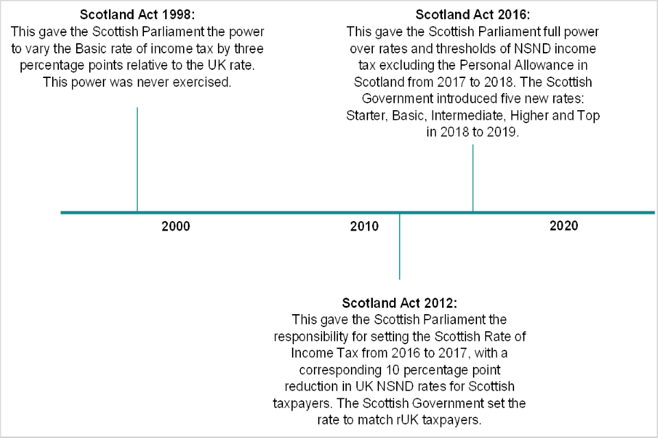
Figure 1 shows a horizontal time axis of 1998 to 2020. There are three spokes along the axis which represent the Scotland Acts of 1998, 2012 and 2016 coming into power. There is a brief description of the powers that each Act granted. For a description of the powers shown in this figure, please refer to ‘The Scotland Acts’ section of the paper above.
5.2 Five-band policy in 2018 to 2019
For the tax year 2018 to 2019 the Scottish Government introduced two new Income Tax bands and their associated rates, as well as increasing the rates for two of the existing bands. This switched Scotland from a three-band system to a five-band system.
Taxpayers in Scotland therefore face five different marginal tax rates beginning with the Starter rate of 19%, a Basic rate of 20%, a new Intermediate rate of 21%, a Higher rate of 41% and a Top rate of 46%. Table 5 below shows the new Scottish Income Tax system for the tax year 2018 to 2019 and Table 6 shows the rUK system for the same year.
Table 5: Scottish Income Tax NSND policy for the tax year 2018 to 2019.
| Tax band | Scottish threshold | Scottish Income Tax marginal rate |
|---|---|---|
| Starter rate | £11,850 | 19% |
| Basic rate | £13,850 | 20% |
| Intermediate rate | £24,000 | 21% |
| Higher rate | £43,430 | 41% |
| Top rate | £150,000 | 46% |
Table 6: rUK NSND Income Tax policy for the tax year 2018 to 2019.
| Tax band | rUK threshold | rUK marginal rate |
|---|---|---|
| Basic rate | £11,850 | 20% |
| Higher rate | £46,350 | 40% |
| Additional rate | £150,000 | 45% |
As can be seen in Tables 5 and 6, a high earning Scottish taxpayer will face a higher marginal Income Tax rate than someone in rUK with the same level of income, while a low earning taxpayer will face a lower marginal rate.
In addition to the five and three-bands in Scotland and the rUK respectively, it’s important to be aware of the Taper rate. For incomes above £100,000, a taxpayer’s Personal Allowance (the first £11,850 of income in 2018 to 2019) is removed by the amount of £1 for every £2 of additional income. In effect, this means that a Scottish taxpayer faces a marginal rate of 61.5% on their earned income between £100,000 and £123,700 while and a rUK taxpayer faces a marginal rate of 60%.
Both groups of taxpayers are subject to the Taper rate given that the Personal Allowance is not devolved, however the marginal rates over the income band are different because Scottish taxpayers are losing their Personal Allowance to a Higher rate of 41% relative to their rUK peers’ Higher rate of 40%.
Figure 2 below shows the differences in the marginal rates faced by different income levels for both Scottish and rUK taxpayers. For the purposes of our study, we are not examining or including the effects of National Insurance Contributions (NICs) which are not devolved to the Scottish Parliament, nor are we considering any other taxes or deductions to income.
Figure 2: Marginal NSND Income Tax rates in Scotland and rUK in the tax year 2018 to 2019.
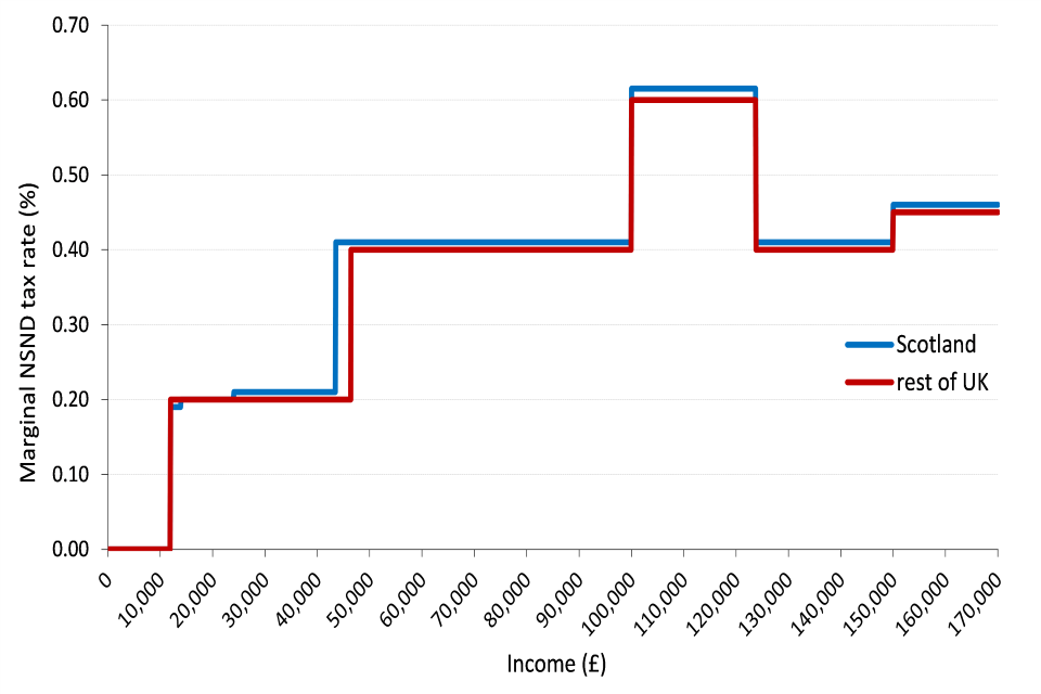
Figure 2 shows taxpayer income along the x-axis with the associated marginal tax rate for Scotland and the rUK along the y-axis. The marginal rates for Scotland are lower or equal to the rUK rates from £11,850 to £24,000, before Scotland has higher marginal rates for incomes greater than £24,000.
Tables 5 and 6 coupled with Figure 2 demonstrate a Scottish taxpayer earning less than £13,850 will have a lower marginal rate compared to a rUK taxpayer on the same income. This means their take home pay for every pound earned in that band, their MRR, will be higher in Scotland. However, a taxpayer earning above £24,000 will face higher marginal rates of Income Tax, and therefore have a lower MRR for each pound of income they earn above that amount in Scotland.
6. Related literature
This section presents literature on TIE studies from a variety of different tax reforms that have taken place in the past. Most of the literature available focuses on reforms in the United States of America (USA), but there are existing studies for tax changes in other countries, including the UK. Note that the literature often refers to TIEs as “Elasticity of Taxable Income” or ETI’s. Elasticities tend to be negligible or very small at the beginning of the income distribution and increase with income.
The literature considers varying behaviour by taxpayers that will affect taxable income in response to a change in the tax rate. Behaviours that reduce taxable income gradually are considered to be ‘intensive’, for example avoidance, reducing hours, or not investing to expand a personal business. Behaviours that remove individuals from the workforce completely such as retirement, not starting a business, or migration are described as ‘extensive’.
Different studies will include different behaviours in their estimated TIEs, but the estimates are still broadly comparable. Generally speaking, extensive effects tend to be much smaller than intensive effects. Since our paper only includes taxpayers remaining resident as a taxpayer in Scotland or rUK across the entire period, we define our estimated TIEs as capturing behaviour along the intensive margin only.
6.1 UK based literature
Brewer, Saez and Shephard (2010) present a top income share analysis for the UK between 1962 and 2003. There were two notable tax changes introduced by the UK Government in this period: the top marginal tax rate was cut from 83% to 60% in 1979 and then reduced to 40% in 1988. They use a difference-in-differences design which relies on the identifying assumption that income growth would have been the same amongst the treatment and control groups. They look at two approaches:
- the change in income share of the top 1% of earners; and
- the change in the top 1% of earners using the next 4% of earners as a control group.
They find elasticities around the 1979 reform between 0.34 when considering the first approach and 0.08 when using the second approach. The elasticities for the 1988 reform are estimated to be between 0.37 and 0.41 for both approaches respectively. Finally, when considering a full time-series regression from 1973 to 2003, they found an elasticity of 0.73 and 0.46 respectively.
HMRC (2012) estimate a TIE using the 2010 to 2011 introduction of the 50% Additional rate of Income Tax. They used a four-step approach to estimating a TIE from SA returns. Whilst their estimates for elasticities ranged between 0.48 and 0.71 when varying their controls, they suggest a TIE of 0.45 as their central estimate when considering the available evidence on TIEs.
The Institute for Fiscal Studies followed up on this research in 2017. They updated HMRC’s approach with an extra year of data and found an elasticity of 0.31 for the Additional rate population based on the response in 2010 to 2011, and 0.83 based on the response in 2011 to 2012. IFS researchers assert that HMRC’s method for estimating the effects of forestalling at the time was “likely to lead to overestimates of how much came from these initial post‑reform years, and hence underestimate the underlying taxable income elasticity” (Browne and Phillips, 2017). They therefore suggested an alternative method which gives them an elasticity of 0.58 for the response of this population in 2010 to 2011 and 0.95 in 2011 to 2012.
6.2 International literature
Feldstein (1995) uses a panel of individual income tax reforms to study the 1986 Tax Reform Act in the USA. This reform reduced the top tax rate from 50% to 28% in 1988. A difference-in-differences strategy is used to estimate a range of elasticities with respect to the net-of-tax rate. Feldstein finds TIEs between 1.10 and 3.05 for high income individuals.
These estimates are similar to the estimates of Lindsey (1987) who studied the 1981 Economic Recovery Tax Act which provided a 23% reduction in tax rates over three years and an immediate cut in the top personal rate from 70% to 50%. Lindsey used non-panel tax return data to give estimates with ranges from 1.05 to 2.75, with most of the data suggesting a TIE between 1.6 and 1.8.
A study on a panel of USA tax returns that Gruber and Saez (2002) analysed throughout the 1980s gives estimates of TIEs according to income level. The top marginal income tax rate at the federal level fell from 70% in 1980 to 28% by 1988, with a reduction from fifteen income tax brackets to four. They estimate the TIE for individuals earning between $10,000 and $50,000 to be between 0.180 and 0.284. They estimate a TIE between 0.106 and 0.265 for individuals with higher earnings in the range of $50,000 to $100,000. Finally, they estimate a TIE between 0.484 and 0.567 for individuals with incomes in excess of $100,000.
Saez (2004) uses USA income tax data from 1960 to 2000 to analyse behavioural responses to taxation. Saez finds that “only the top 1% incomes show evidence of behavioural responses to taxation”. This study argues that there was no response to the large top rate cuts in the early 1960s but there has been evidence of responses since the 1980s. Saez uses a time-series regression to find elasticity estimates between 0.50 and 0.71 when accounting for time trends.
Saez, Slemrod and Giertz (2012) use difference-in-differences to estimate elasticities for the top 1% and the next 9% of incomes. This is performed across four individual tax changes as well as across a time series from 1960 to 2006. Across the full time-series regression, they find an elasticity ranging from 1.71 with no time trends to 0.58 with time trends for the top 1% of incomes. By contrast, the next 9% have coefficients that are roughly zero which supports the findings of Saez’s 2004 paper.
Studies of tax reforms in Nordic countries by Aarbu and Thoresen (2001) and Kleven and Schultz (2014) find lower TIE estimates. Aarbu and Thoresen studied the 1992 tax reform in Norway which increased the MRR for high-income earners using a difference‑in-differences approach. They find relatively low elasticities with respect to the net-of-tax rate by comparison to USA studies, ranging from -0.6 and 0.2.
Similarly, Kleven and Schultz use Danish population data beginning in 1980 covering four separate reforms, the largest of which occurred in 1987 where the marginal tax rate for high and middle earners was reduced. They found that the TIEs across all reforms considered are approximately 0.082 but increase to 0.189 for the 1987 reform.
Table 7: Summary table of literature.
| Name of Paper | Tax base | TIE |
|---|---|---|
| Brewer, Saez and Shepherd (2010) | Top 1% of UK taxpayers | 0.34 |
| HMRC (2012) | Additional rate UK taxpayers | 0.45 |
| Browne and Phillips (2017) | Additional rate UK taxpayers | 0.58 |
| Lindsey (1987) | USA incomes of at least $100,000 | 1.02 |
| Feldstein (1995) | High income USA taxpayers | 1.10 to 3.05 |
| Gruber and Saez (2002) | USA incomes of at least $100,000 | 0.484 to 0.567 |
| Saez (2004) | USA incomes of top 1% | 0.5 to 0.71 |
| Saez, Slemrod and Giertz (2012) | USA incomes of top 1% | 0.58 to 1.71 |
| Aarbu and Thoresen (2001) | Norway high incomes | -0.6 and 0.2 |
| Kleven and Schultz (2014) | All Danish taxpayers | 0.082 to 0.189 |
7. Data
7.1 Taxpayer data sources
We have drawn upon HMRC’s RTI data for Pay-As-You-Earn (PAYE) taxpayers. This data is submitted to HMRC by employers whenever they make a payment to their staff. It includes the amount of money paid to the employee, the Income Tax withheld from them on behalf of HMRC and the necessary information to identify the taxpayer, such as their national insurance number (NINO).
For SA taxpayers, we have drawn upon the data extracted annually by HMRC to produce the Scottish Income Tax Outturn Statistics. Specifically, our SA dataset is consistent with the established or known Scottish Income Tax liabilities at the time the outturn was produced. Some liabilities for any given year can be collected several months or years after the fiscal year has ended. This unestablished amount is estimated in the Outturn Statistics based on historical data and makes up approximately 1% of all liabilities. For our purposes we only require those taxpayers with confirmed liabilities to be able to study their behaviour. We do not believe the absence of the unestablished amount will impact our results.
Both our RTI and SA datasets include pensioners in addition to the active workforce, since pension income is included under NSND income. The datasets cover taxpayers from the whole of the UK.
For our study we have used data from the three tax years of 2016 to 2017, 2017 to 2018 and 2018 to 2019. This enables us to estimate the behavioural response in the final year when the five-band policy was introduced, known as the treatment year, as well as draw upon the trends in taxpayer incomes before that year to use in our methodology.
Our dataset only includes taxpayers present in all three tax years, known as a balanced panel dataset, and it excludes any taxpayers who moved from Scotland to the rUK during that time, or vice versa.
7.2 Income variable
NSND income is the primary variable in our data set. For PAYE, an individual’s annual NSND income is assumed to be the sum of their monthly pay across the tax year. Where they have multiple pay amounts per month, for example someone who has two or more employments, these have been summed under the same individual and included in their total pay. This is because Income Tax liabilities are calculated on a person’s total income, not on an employment-by-employment basis such as under the NICs policy.
Our RTI datasets cover the full payment submissions reported for employees from April 2016 to March 2017 for the tax year 2016 to 2017, and the equivalent time period for the other two tax years.
For SA, an individual’s annual NSND income is readily available from the SA outturn data. For the tax year 2016 to 2017 this includes all SA returns captured by the filing deadline of April 2018, and by the equivalent deadline for the other two tax years.
Employed individuals who paid Income Tax via the PAYE collection method and thus appear in RTI may also have been required to file an SA return. This is because SA returns are not solely for the self-employed. An employed individual may have to file for several reasons, including earning over £100,000 in any given year or having an employed income and a self-employment income.
For individuals with both an RTI record and an SA record, we have prioritised their SA income over their RTI pay in any given year. Their SA NSND income will capture all forms of income, including their employment income from RTI. We have therefore sought to ensure that each individual taxpayer only has one income record in our dataset.
7.3 Scottish Indicators (s-flags)
The definition of a Scottish taxpayer is based on where an individual resides for the majority of a tax year. Scottish taxpayer status applies for a whole tax year – it is not possible to be a Scottish taxpayer for part of a tax year. The location of a person’s employer is not relevant. For example, someone who works in Scotland but has their main home elsewhere in the UK will not be a Scottish taxpayer. Further information on who pays Scottish Income Tax can be found on the GOV.UK website.
Once a Scottish taxpayer has been identified they are given a Scottish indicator, often referred to as an s-flag, which means they have paid their Income Tax liabilities under the five-band Scottish regime, not the three-band rUK regime. We use this s-flag variable to identify our Scottish taxpayers in the tax year 2018 to 2019 in our treatment group.
The s-flags in our dataset for both RTI and SA taxpayers are drawn from, and therefore consistent with, the HMRC data used to construct the Scottish Income Tax Outturn Statistics.
7.4 Demographic variables (Age, Sex and Sector)
We have sourced taxpayer age from HMRC’s RTI data for both RTI and SA taxpayers wherever possible. This is taken as their age at the end of the tax year in question. We have also sourced taxpayer sex from the same RTI data source for both RTI and SA taxpayers. This will be the sex provided to HMRC by their employer.
For sector and industry classification we have applied the relevant Standard Industrial Classification of Economic Activities (SIC) codes from 2007 to our taxpayers wherever possible and placed these into the twenty-one sections of industry ranging from Agriculture, Forestry and Fishing (A) to Activities of extra territorial organisations and bodies (U). A full list of the twenty-one sections of industry can be found on the Companies House website.
For RTI taxpayers we have sourced a SIC code that is assigned to each taxpayer based on their employment. For a taxpayer with multiple employments, we have taken the SIC code attached to their employment with the highest amount of pay in that year. The exception to this is when an RTI taxpayer’s record is flagged as being from an occupational pension. All RTI records are flagged as either employment pay or occupational pension pay. If flagged as the latter, the RTI taxpayer is classified as a Pensioner and not their industry classification.
For SA taxpayers, a taxpayer’s main source of income is the factor that determines their industry classification. For example, for an SA taxpayer whose main source of income is classified as employment pay, we have sourced a SIC code on record based on their employer. For an SA taxpayer whose main source of income is classified as being a sole trader, we have sourced their SIC code on record based on their trade income. For each of these SIC sources, there may be missing information for some taxpayers. Table 8 below sets out the different classifications of SIC code for our SA taxpayers.
Table 8: SIC code source for SA taxpayers.
| Main Source of Income Classification | Associated SIC Source |
|---|---|
| Pay | Employer SIC code |
| Sole Trader | Trade SIC code |
| Partnership | Partnership SIC code |
| Occupational Pension or anyone with income from Pensions irrespective of their Main Source | Pensioner |
In the instances where a taxpayer has both an RTI SIC code and an SA SIC code, we have prioritised their SA SIC code for all taxpayers with one exception. This being that if they have a main source classification of employment pay and their SA SIC code is missing, we have allowed for their RTI SIC code to replace their missing SA SIC code. Where it is not missing, their SA SIC code still takes priority for any main source classifications of employment pay.
Finally, Table 9 below summarises the sources for our key variables.
Table 9: Summary of sources for key variables in our dataset.
| Variable | Source |
|---|---|
| Income | Real Time Information (RTI) and Self-Assessment (SA) Outturn data |
| Scottish Indicators (s-flags) | Scottish Income Tax Outturn data |
| Age | RTI data |
| Sex | RTI data |
| Sector and Industry | RTI and SA data |
8. Descriptive Statistics
8.1 Taxpayer Statistics
The statistics presented here are for the population used in our analysis. Migrants between Scotland and rUK have been removed and the panel is balanced so that each individual appears in all three tax years. While these figures consider all individuals within Scotland and rUK, some individuals will be omitted by the econometric methodology.
8.2 Number of taxpayers in each band for 2017 to 2018
Table 10 presents the number of taxpayers in each income band for 2017 to 2018. We see that the majority of taxpayers considered have income between £11,850 and £43,430 (84%). There are approximately 15.5 million individuals who have income below the Personal Allowance. These individuals are dropped from the analysis and are not included in any other figures or tables. Numbers are rounded to the nearest 500.
Table 10: Number of people in each income band for the whole of the UK in 2017 to 2018.
| Income Band | Income Range | Number of people in 2017 to 2018 | Proportion of individuals (%) |
|---|---|---|---|
| 0 | Below £11,850 | 15,828,500 | 37.7 |
| 1 | £11,850 - £13,850 | 2,353,500 | 5.6 |
| 2 | £13,851 - £24,000 | 10,479,000 | 25.0 |
| 3 | £24,001 - £43,430 | 9,097,000 | 21.7 |
| 4 | £43,431 - £80,000 | 3,093,000 | 7.4 |
| 5 | £80,001 - £100,000 | 413,000 | 1.0 |
| 6 | £100,001 - £123,700 | 247,000 | 0.6 |
| 7 | £123,701 - £150,000 | 143,500 | 0.3 |
| 8 | £150,001 - £300,000 | 231,500 | 0.6 |
| 9 | £300,001 - £500,00 | 54,500 | 0.1 |
| 10 | £500,000+ | 43,500 | 0.1 |
Figure 3: Number of taxpayers in each income band for 2017 to 2018.
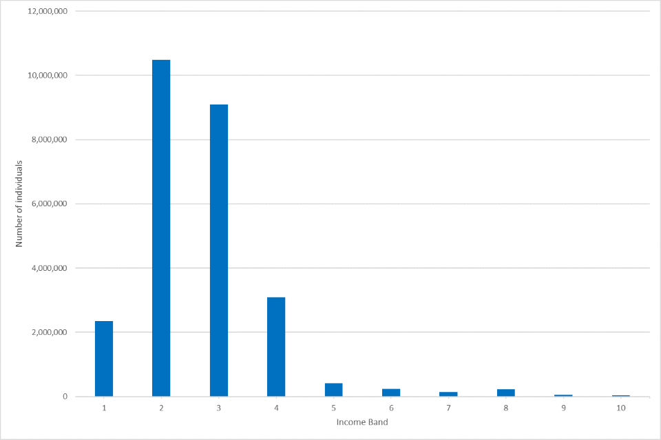
This figure shows the distribution of taxpayers across the income bands. There are roughly 2 million individuals in income band 1, which increases to around 10m in income band 2. Beyond this point, the number of individuals falls a small amount for band 3 followed by a substantial drop in income band 4 and beyond.
8.3 Taxpayers across rUK and Scotland
The distribution of taxpayers across the income bands is relatively similar in rUK and Scotland. There is a slightly smaller proportion of individuals in the Basic rate in rUK than in Scotland, and this is reflected by having a slightly larger proportion of individuals that are in the Higher and Additional / Top rate bands.
Figure 4: Distribution of taxpayers according to income band in rUK and Scotland.
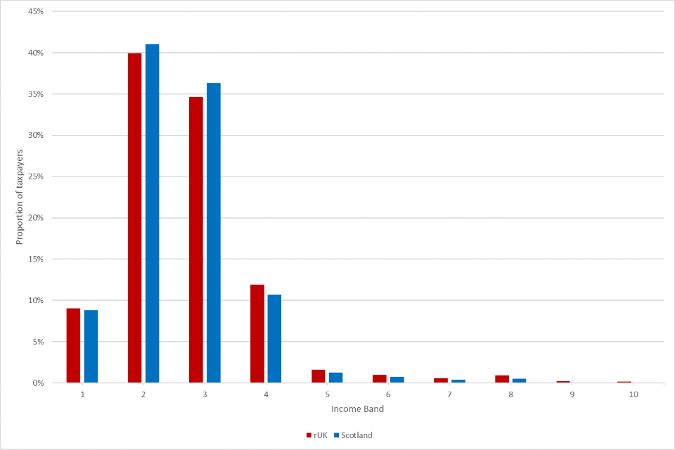
This figure compares the distribution of incomes across rUK and Scotland. Overall, the shapes of the distributions are similar, with the largest proportions of individuals in income bands 2 and 3. There are very small differences across distributions in rUK and Scotland, with Scotland having more individuals in income bands 2 and 3, but fewer in the higher income bands.
8.4 Age Distribution
There are some differences in the age distribution for taxpayers in Scotland and rUK. The latter has a greater proportion of people between the ages of 20 and 40 years. The figures are similar for the 40 to 50 year age group. Scotland then has a larger proportion of individuals aged between 50 and 70 years. And finally, rUK has slightly more individuals (as a proportion) that are aged 70 and over.
Figure 5: Age Distribution across rUK and Scotland.
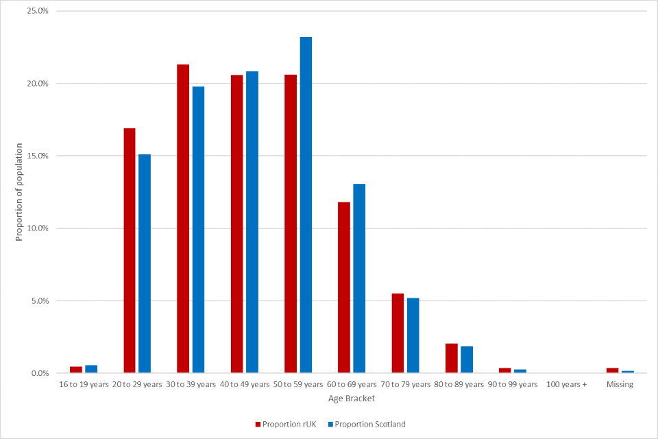
This figure describes the distributions across Scotland and rUK. rUK has more individuals between the ages of 20 to 40 years, whereas Scotland has more people between the ages of 50 and 70 years.
8.5 Sex Distribution
The following table captures the sex of individuals for Scotland and rUK. The proportion of people that are male is larger in rUK than in Scotland for the population captured within our analysis.
Table 11: Distribution of sex across rUK and Scotland.
| Sex | rUK (%) | Scotland (%) |
|---|---|---|
| Female | 41.9 | 43.2 |
| Male | 57.7 | 56.6 |
| Missing | 0.4 | 0.2 |
8.6 Sectoral Distribution
The distribution of sectors between rUK and Scotland tends to be fairly similar as shown by the figure below. The dominant sector recorded is the public sector for both rUK and Scotland and the second most dominant sector is pensions. The public sector is constructed using a combination of “Public Administration”, “Education” and “Human Health”. We acknowledge that there may be individuals within these groups that are in the private sector and that there may be individuals in the public sector not captured in these groups.
Figure 6: Distribution of sectors across rUK and Scotland.
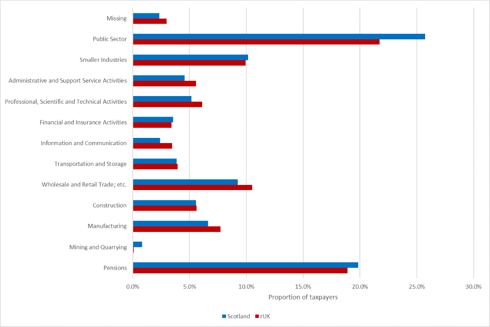
This figure compares the distributions of taxpayers across sectors within Scotland and rUK. The majority of individuals are in the public sector, with the second largest sector being pensions. Scotland has much larger proportions of individuals in the public sector, pensions and mining and quarrying. rUK has larger proportions within Wholesale and Retail Trade, Administrative and Support Service Activities and Manufacturing. All other sectors have roughly equal proportions of individuals.
8.7 Macroeconomic Trends
8.8 GDP Growth
ONS data is used to construct GDP growth trends between Scotland and rUK (Extra-Regio activity has been removed). Typically, GDP growth has been stronger in rUK since 2010. The ONS figures of regional GDP growth are broadly similar to those produced by the Scottish Government, and allow for comparable figures for Scotland and the rUK.
Figure 7: GDP Growth across Scotland and rUK.
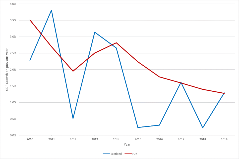
This figure shows a comparison of GDP growth between Scotland and rUK from 2010 to 2019. GDP growth in rUK is much more stable, with growth generally falling since 2014. In Scotland, there is volatility in the GDP growth rate, which repeatedly goes from high to low.
8.9 Employment rate
Labour Force Survey (LFS) data is used to construct a comparison of employment for Scotland and rUK. The employment rate (defined as the proportion of the population over 16 in employment) has typically been lower in Scotland.
Figure 8: Employment rate trends across rUK and Scotland.
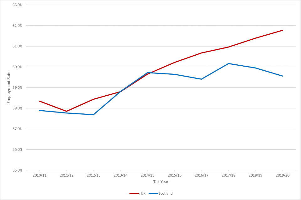
This figure shows the changes in employment rates over time per tax year for Scotland and rUK from 2010 to 2011 up to 2019 to 2020. The employment rate in rUK has been steadily increasing from around 58% in 2011 to 2012 up to 62% in 2019 to 2020. In Scotland, there is a similar upward trend until 2014 to 2015. There is then a divergence, where employment rates become flatter and are close to 60% up to 2019 to 2020.
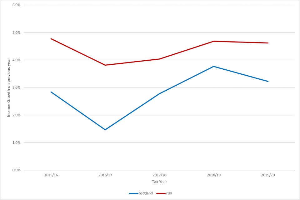
8.10 Pay Growth
The following is taken from RTI data, showing the trend of pay growth for employees between Scotland and rUK. RTI pay has grown faster by approximately 1 to 2 percentage points in rUK compared to Scotland since the tax year 2015 to 2016.
Figure 9: Pay Growth Trends.
9. Methodology
We use propensity score matching and difference-in-differences to estimate the percentage change in taxable income for Scottish taxpayers as a result of the policy. Our design takes advantage of Income Tax changes in Scotland by comparing Scottish taxpayers to a matched control group from rUK. We recover the Average Treatment Effect on the Treated (ATET), or in other words, the impact on NSND income declared by Scottish taxpayers facing new Income Tax rates in 2018 to 2019.
Our methodology selects a control group from rUK who match Scottish taxpayers in key dimensions, including historical income growth and sector. We difference the mean log change in income between the treatment and control groups to recover the policy effect. Using this approach, we estimate the average percentage change in income in Scotland without specifying a functional form.
Individuals are grouped into income bands reflecting their marginal rate to allow estimation of the different behaviour of taxpayers at different income levels (heterogeneous behaviour). Cross-border migrants are excluded from the analysis. In this way the identified parameter reflects the intensive behavioural margin, which captures behaviour relating to the amount of income declared rather than other behaviours such as migration from Scotland.
9.1 Behavioural Effects
To identify the policy effect, we assume individuals only react to changes in their marginal tax rate. Equivalently, as in Saez et al. (2012), we assume income effects do not generate behaviours to reduce taxable income. This assumption is important to account for the many tax rate changes individuals face below their margin that influence net-of-tax-income.
We define the MRR as one minus the marginal Income Tax rate. This variable summarises the behavioural incentives faced by individuals. It reflects the amount of income available to spend after tax. Our definition excludes NICs, tuition fees, and various other deductions.
We split the population into ten bands and restrict the treated groups such that individuals are only compared to others experiencing the same proportional change in their MRR. The relative change in the MRR varies across tax bands since we calculate the change in the MRR as the difference in natural logarithms of the post and pre-policy MRR:
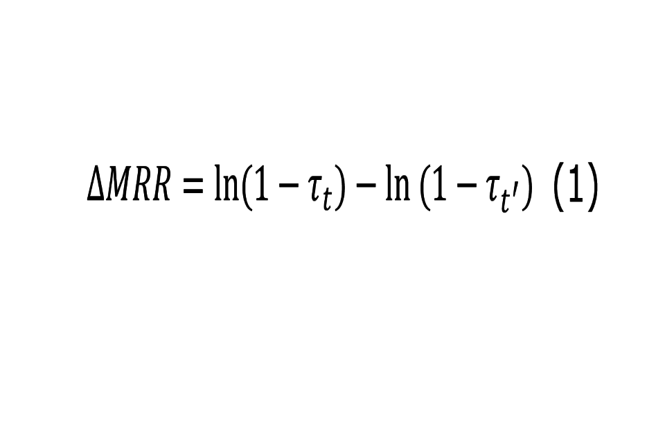
Formula: The change in the MRR is equal to the difference in natural logarithms of the post and pre policy MRR.
Where τt’ and τt are the marginal tax rates before and after the policy change respectively. For example, in the Additional / Top rate a change in MRR from 0.55 to 0.54 imposes a fall of 1.8%, whereas in the Intermediate rate a change from 0.8 to 0.79 imposes a fall of only 1.3%. In effect, the Additional / Top rate experiences a different policy change to the Intermediate rate.
We allocate individuals into ten income bands according to their income in the 2017 to 2018 tax year. The ten income band structure reflects the five-band system, with logical points for changes in the MRR such as the Taper rate, and is consistent with the Scottish Fiscal Commission’s behavioural framework for splitting up the Additional / Top rate. This allows us to capture heterogeneity in responses.
Table 12: Income bands used for TIEs analysis.
| Income Band | Lower Threshold | Upper Threshold | MRR before tax change | MRR after tax change |
|---|---|---|---|---|
| 1 – Starter Rate | Personal Allowance (£11,850) | £13,850 | 80% | 81% |
| 2 – Basic Rate | £13,851 | £24,000 | 80% | 80% |
| 3 – Intermediate Rate | £24,001 | £43,430 | 80% | 79% |
| 4 – Low Higher Rate | £43,431 | £80,000 | 60% | 59% |
| 5 – Medium Higher Rate | £80,001 | £100,000 | 60% | 59% |
| 6 – Personal Allowance Taper | £100,001 | £123,700 | 40% | 38.5% |
| 7 – Upper Higher Rate | £123,701 | £150,000 | 60% | 59% |
| 8 – Low Top Rate | £150,001 | £300,000 | 55% | 54% |
| 9 – Medium Top Rate | £300,001 | £500,000 | 55% | 54% |
| 10 – Upper Top Rate | £500,000 | Unbounded | 55% | 54% |
Cross-border migrants are removed from the dataset. It is possible that the decision to migrate is influenced by tax policy. Excluding migrants at the same time as the policy change is a decision to exclude part of the behavioural effect from the identified parameter. This aligns the recovered estimate of the behavioural effect more closely to the intensive margin.
9.2 Difference-in-Differences Matching Model
A difference-in-differences methodology compares the change in income before and after the policy between the treated and control groups. The control group provides us with a counterfactual difference – the change we would expect in the absence of a policy impact. This is valid on the assumption that, in the absence of the policy, income would change at the same rate, often called the ‘parallel’ or ‘common’ trends assumption. This approach controls for selection on fixed effects, and changes that are common to both groups.
Scotland and rUK are divergent in key dimensions. Historically, income grows at significantly different rates for the two countries as can be seen by Figure 9 of the descriptive statistics showing RTI pay growth. To attempt to control for non-parallel trends, we select a control group using propensity score matching. This technique allows us to compare Scottish taxpayers with taxpayers from rUK who are similar in terms of key characteristics. A propensity score is the probability of treatment given a vector of observable variables.
We estimate propensity scores using a logistic (logit) regression. Historical income growth rates, the log of current income, sex, sector, and age act as covariates. Historical growth is defined as the difference in the log of income between 2016 to 2017 and 2017 to 2018.
Individuals are matched on tax year 2017 to 2018, the year before the policy change. Matches are restricted to within income band. By matching on historical growth, we create a re-weighted control group that is more likely to be on a parallel trend across the pre-reform periods in the dataset.
The study presents three alternative methods when matching treated individuals with those in the control group: (1) nearest neighbour with one-to-one matching; (2) nearest neighbour with one-to-two matching; and (3) kernel matching.
The nearest neighbour matches are with replacement. For Kernel matching we use an Epanechnikov kernel function and automatically compute the bandwidth as per Jann (2017). We bootstrap standard errors for kernel matching and use Abadie and Imbens (2006) to calculate standard errors for nearest neighbour matches.
Our headline estimates are taken from (1) nearest neighbour with one-to-one matching but no single method is clearly preferable. Therefore, the analysis presents all three to test the robustness of the observed treatment effects.
The ATET is a weighted average of the difference in continuous growth rates between individuals in the treatment and the control groups. It is obtained by estimating the following equation (Lenhart, 2019):
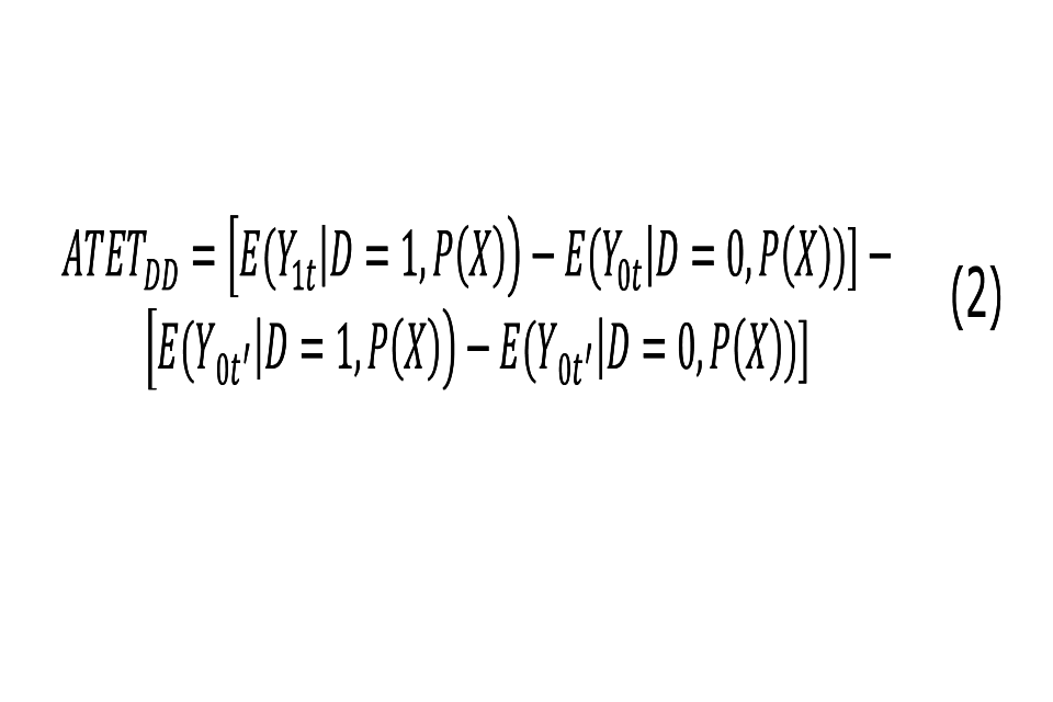
Formula: The difference in expected outcome for the treated and control groups after the policy, minus the difference in expected outcomes before the policy, conditional on propensity score.
D=1 indicates treatment and D=0 indicates non-treatment, P(X) denotes the propensity score, Y is income for an individual where subscript 0 denotes the untreated state, subscript 1 denotes the treated state, subscript t denotes the post-treatment period and subscript t’ denotes the pre-treatment period.
From Heckman et al. (1997), the estimator above identifies the average treatment effect on the treated if the following assumption holds:
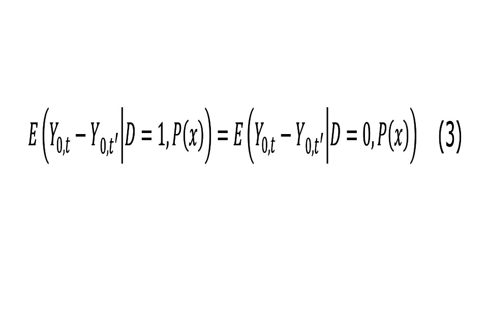
Formula: Income growth for the treated group would equal income growth in the control group if tax rates had not changed, conditional on propensity score.
The recovered statistic is the percentage change in income caused by policy. This is converted to an elasticity by dividing by the change in MRR. The individual is assumed to react to changes in their headline rate of tax, and we do not account for idiosyncratic factors that might influence an individual’s effective rate, such as switching income bands. The formula for the conversion is given below.
Formula: The conversion calculates the taxable income elasticity given the ATET. The difference in log income before and after implementation is divided by the difference in log MRR before and after implementation.
Where the ATET is the treatment effect defined above, (1-τ) is the MRR, the subscript t denotes the post-treatment period and the subscript t’ denotes the pre-treatment period.
10. Results
Our headline estimates are nearest neighbour with one-to-one matching. The ATET captures the average percentage change in income for a given income band as a result of the tax change in Scotland.
10.1 Percentage Changes in Income
Table 13: Average treatment effect on the treated across all income bands.
| Income Band | Income Range | Nearest Neighbour (1) | Nearest Neighbour (2) | Kernel |
|---|---|---|---|---|
| Band 10 | £500,000 + | -0.100**, (0.0427) | -0.0695*, (0.0376) | -0.0530, (0.0451) |
| Band 9 | £300,001 - £500,000 | -0.0438, (0.0275) | -0.0346, (0.0231) | -0.0161, (0.0220) |
| Band 8 | £150,001 - £300,000 | -0.00326, (0.00975) | -0.00872, (0.00837) | -0.0125*, (0.00673) |
| Band 7 | £123,701 - £150,000 | -0.00205, (0.00919) | 0.000705, (0.00811) | -0.00492, (0.00723) |
| Band 6 | £100,001 - £123,700 | -0.0111, (0.00675) | -0.0166***, (0.00586) | -0.0177***, (0.00582) |
| Band 5 | £80,001 - £100,000 | -0.00448, (0.00455) | -0.00671*, (0.00396) | -0.00670, (0.00461) |
| Band 4 | £43,431 - £80,000 | -0.00588***, (0.00125) | -0.00526***, (0.00108) | -0.00548***, (0.00123) |
| Band 3 | £24,001 - £43,430 | 0.00306***, (0.000601) | 0.00325***, (0.000512) | 0.00318***, (0.000539) |
| Band 2 | £13,851 - £24,000 | No Tax Change | No Tax Change | No Tax Change |
| Band 1 | £11,850 - £13,850 | -0.000734, (0.00165) | 0.0000948, (0.00142) | 0.00129, (0.0018926) |
Standard errors in parentheses. *** p<0.01, ** p<0.05, * p<0.1
10.2 TIEs
This section shows the results above as TIEs with respect to the MRR.
Table 14: Taxable income elasticities.
| Income Band | Income Range | Nearest Neighbour (1) | Nearest Neighbour (2) | Kernel |
|---|---|---|---|---|
| Band 10 | £500,000 + | 5.45** | 3.79* | 2.89 |
| Band 9 | £300,001 - £500,000 | 2.39 | 1.89 | 0.88 |
| Band 8 | £150,001 - £300,000 | 0.18 | 0.48 | 0.68* |
| Band 7 | £123,701 - £150,000 | 0.12 | -0.04 | 0.29 |
| Band 6 | £100,001 - £123,700 | 0.29 | 0.43*** | 0.46*** |
| Band 5 | £80,001 - £100,000 | 0.27 | 0.40* | 0.40 |
| Band 4 | £43,431 - £80,000 | 0.35*** | 0.31*** | 0.33*** |
| Band 3 | £24,001 - £43,430 | -0.24*** | -0.26*** | -0.25*** |
| Band 2 | £13,851 - £24,000 | No Tax Change | No Tax Change | No Tax Change |
| Band 1 | £11,850 - £13,850 | -0.06 | 0.01 | 0.10 |
*** p<0.01, ** p<0.05, * p<0.1
11. Robustness Checks
11.1 Balancing Tests
Standardisation Bias
The quality of matching is assessed by performing tests that check whether the propensity score adequately balances the characteristics of the treatment and control groups. We test the matching quality by using the standardised bias as suggested by Rosenbaum and Rubin (1985). It is defined as the difference of sample means in the treatment and matched control subsamples as a percentage of the square root of the average of sample variances in both groups for each covariate. The standardised bias after matching is given by:
Formula: The bias is the difference in means between the treated and control group covariate, divided by the square root of half the total variance, multiplied by 100.
Where X1 (V1) is the mean (variance) in the treatment group after matching and X0 (V0) is the analogue for the control group. Many empirical studies regard a standardisation bias of less than 5% as sufficient.
We generally find that the standardisation bias between the treatment and matched control groups is less than 5% in most cases. This holds true for all income bands, regardless of whether we use nearest neighbour or kernel matching.
T-test difference of means
T-tests are used to check for the equality of covariate means in the treatment and matched control group. If there is good balance, then there will not be statistically significant differences between the means of the covariates. We consider these tests at the 5% significance level.
We find that in most cases, there are no statistically significant differences at the 5% level between the means of the treated and control groups. These results hold across income bands and matching methods. The t-tests and standardisation bias reinforce the strength of our results and show that there is generally good balance in the propensity score matching methodology.
11.2 Overlap Condition
A further check on propensity score matching is to verify the overlap condition. The idea here is to visually inspect the propensity score distributions for both the treatment and control groups, looking at the closeness of the overlap. There should be no clear or sizeable differences between the treatment and control groups after the matching process. All graphs are shown in Annex B (when considering nearest neighbour with one‑to-one matching).
Figure 10: Propensity score overlap before and after matching for income band 1, with nearest neighbour one-to-one matching.

Figure 10 shows the propensity scores before and after matching for income band 1 with nearest neighbour one-to-one matching. On the left, the graph shows the density of propensity scores for the treated and control groups before matching, where we see that there are sizeable differences in the density of propensity scores. On the right we see overlap between the treated and matched control groups.
Figure 11: Propensity score overlap before and after matching for income band 10, with nearest neighbour one-to-one matching.
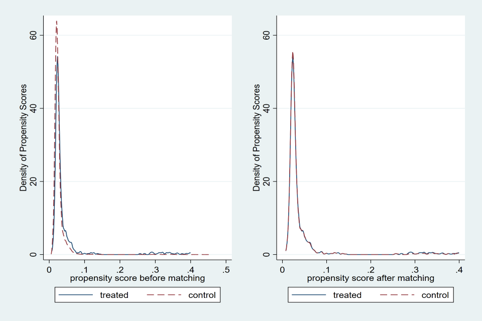
Figure 11 shows a comparison of the density of propensity scores before and after matching for income band 10, with nearest neighbour one-to-one matching. The left‑hand side shows the comparison of propensity scores before matching, showing a clear difference in the peak of propensity scores for the treated and control groups. The right-hand side shows the comparison of propensity scores after matching and shows that there is very little difference between the densities of propensity scores.
The graphs show how the matching process improved the overlap of the control group. The left-hand side of figures 10 and 11 compare everyone in rUK within the respective income band in the control group to Scottish taxpayers. Before matching, the shape of the densities are similar, but the peak and range of propensity scores are much higher for the control group. The post-match graphs show how matching has improved the fit of propensity scores in the control group to Scotland. In all cases across all income bands, the overlap between treated and control groups is improved by the match.
11.3 Alternative Specifications
We investigated the effects of changing parts of the matching process and including migrants. Overall, there is no major difference to the results when making changes to the matching process. When using a probit regression rather than a logit regression to estimate the propensity scores (with nearest neighbour one-to-one matching) the magnitude of results is generally lower in absolute value. The elasticities generated by using probit regressions follow the same pattern as the headlines, where they increase with income bands. The most notable divergences in elasticities occur in income bands 9 and 10, where the elasticities generated using a probit model to estimate propensity scores are much smaller than those produced by the logit model.
Table 15: Comparison of elasticities under logit and probit models, with nearest neighbour one-to-one matching.
| Income Band | Logit | Probit |
|---|---|---|
| 1 | -0.06 | 0.08 |
| 3 | -0.24 | -0.23 |
| 4 | 0.35 | 0.16 |
| 5 | 0.27 | 0.36 |
| 6 | 0.29 | 0.26 |
| 7 | 0.12 | 0.07 |
| 8 | 0.18 | 0.30 |
| 9 | 2.39 | 0.74 |
| 10 | 5.45 | 2.78 |
The headline results for nearest neighbour matching allow for replacement, where one individual in the control group can be used as a match for multiple treated individuals. Matching can also be performed without replacement, where one individual in the control group can only be matched with one individual in the treatment group. The findings remain consistent when not allowing for replacement. There are only two cases where this makes a large difference to the elasticity, for income bands 7 and 8.
Table 16: Comparison of elasticities for nearest neighbour with one-to-one matching with and without replacement.
| Income Band | With Replacement | Without Replacement |
|---|---|---|
| 1 | -0.06 | -0.03 |
| 3 | -0.24 | -0.22 |
| 4 | 0.35 | 0.30 |
| 5 | 0.27 | 0.35 |
| 6 | 0.29 | 0.36 |
| 7 | 0.12 | -0.05 |
| 8 | 0.18 | 0.51 |
| 9 | 2.39 | 2.34 |
| 10 | 5.45 | 5.23 |
The headline analysis removes all individuals who migrated between Scotland and rUK for the whole period considered. When looking at individuals who migrated between 2016 to 2017 and 2017 to 2018, which consists only of a small number of individuals, we found that this did not make any significant difference to the results.
The final check is on different combinations of covariates used for matching. Our headline analysis uses demographic and income covariates, but we explored using demographics and income alone. We found that there were some larger differences in results compared to our headlines, and that the balance of the specifications was sometimes worse after matching than before matching. The strongest results for balance came from using all covariates.
12. Discussion
The results indicate a range of behavioural effects broadly consistent with the literature. For individuals with income above the Scottish Higher rate threshold, we find a divergence in income growth between the treated and control groups after the policy was implemented.
This implies that above a certain income, individuals in Scotland lowered their taxable income in response to the policy. The size of the response is plausible and generally increasing with income band. The three matching approaches are consistent with one another, and across bands.
Most results are not statistically significant at the 10% level using adjusted standard errors. Although significance does range, no Higher or Additional / Top rate income band is significant across all three matching approaches other than band 4.
We conclude that there is little to no evidence of a behavioural effect for Starter, Basic or Intermediate rate taxpayers. The headline result does show a divergence in income growth between the treated and control groups. However, we test this using band 2 as a placebo and find evidence of a confounding factor. We use a proxy to control for public sector pay. This intuition reflects higher public sector pay growth in Scotland compared to the UK as a whole and is observed in our Basic and Intermediate rate results.
Comparing significance and the validity of the results across income bands is difficult since the size of the treated and control groups vary. Larger sample sizes typically cause smaller confidence intervals and this makes it more likely that we see statistically significant results. We believe this to be the case in lower income bands, since over 84% of taxpayers have incomes between £11,850 and £43,430.
Within our dataset there are only approximately 1,100 treated individuals in band 10, and only 1,800 in band 9. This rises to 10,500 for band 8. Notably, of the Higher rate bands, band 4 is the most consistently significant and has considerably more observations at 216,000. With any analytical study, an estimate based on a small population size can be more susceptible to uncertainty and volatility.
The results satisfy the key tests for validity. They are balanced, with low standardisation bias and t-tests that are not statistically significant. The propensity score overlap between groups show the matching process was successful. These results are relatively invariant to the modelling decisions of the PSM design.
12.1 Top Rate and Additional Rate Taxpayers
Individuals in the Scottish Top rate see a fall in their MRR of 1.8%. Those in band 10 with incomes greater than £500k show the highest potential response, with taxable income falling between 5% and 10%. The response falls with income band: band 9 has a fall between 1.6% and 4.4%, band 8 has a fall between 0.3% and 1.3%. The following table shows the elasticities for each matching approach:
Table 17: TIEs for the Top and Additional rate income bands.
| Band Number | Lower Threshold | Upper Threshold | Nearest Neighbour (1) | Nearest Neighbour (2) | Kernel (Epan) |
|---|---|---|---|---|---|
| 10 | £500,000 | Unbounded | 5.45** | 3.79* | 2.89 |
| 9 | £300,001 | £500,000 | 2.39 | 1.89 | 0.88 |
| 8 | £150,001 | £300,000 | 0.18 | 0.48 | 0.68* |
| All AR | £150,001 | Unbounded | 0.52 | 0.54 | 0.77** |
We find a range of elasticates comparable to similar research from the literature across the entire Top and Additional rate. For comparison, the 2012 HMRC evaluation of the 50% Additional rate estimated elasticities of 0.48 and 0.71. This is also comparable to estimates produced by IFS researchers (Browne and Phillips, 2017) and Brewer et al. (2010).
We note that the elasticities produced by income bands 9 and 10 appear higher than the estimates given in the literature. These results are limited in their interpretation, as they are sensitive to the choice of model to estimate propensity scores. When using probit rather than logit models, we see the elasticities under nearest neighbour with one-to-one matching fall to 0.74 for income band 9 and 2.78 for income band 10. It is intuitive that higher income bands see a greater reaction to tax changes. However, the small number of observations in these groups make the estimation of the elasticity less precise.
When compared to the literature on changes in USA tax policy, the elasticities produced are quite similar despite the differences in fiscal systems. The results are clearly lower than the estimates produced by Feldstein (1995) and Lindsey (1987) but are much more comparable to the studies by Saez (2004) and Saez et al. (2012) where elasticities were between 0.5 to 0.7 when accounting for time trends in the time-series regressions.
The literature in other countries suggests lower elasticities with respect to the MRR. For example, Aarbu and Thoresen’s 2001 study of the 1992 Norwegian tax reform produced elasticity estimates of between -0.6 and 0.2, which are substantially lower than the elasticities estimated within this paper and other studies from the USA.
12.2 Higher Rate Taxpayers
The tax affairs for those in the Higher rate are complicated by the existence of the Personal Allowance Taper, where for every £2 of income above £100,000, the Personal Allowance falls by £1. For bands 4, 5, and 7 the policy increases the marginal rate from 40% to 41%, resulting in a 1.7% fall in the MRR.
However, those with income falling within the Taper rate band face a further marginal change. The Taper rate of 50% means that each pound earned at the margin is effectively taxed at 60% before the policy and 61.5% after the policy. This corresponds to a fall in the MRR of 3.75%. Consider the elasticities in the table below.
Table 18: TIEs for the Higher rate income bands.
| Band Number | Lower Threshold | Upper Threshold | Nearest Neighbour (1) | Nearest Neighbour (2) | Kernel (Epan) |
|---|---|---|---|---|---|
| 7 | £123,701 | £150,000 | 0.12 | -0.04 | 0.29 |
| 6 | £100,001 | £123,700 | 0.29 | 0.43*** | 0.46*** |
| 5 | £80,001 | £100,000 | 0.27 | 0.40* | 0.40 |
| 4 | £43,431 | £80,000 | 0.35*** | 0.31*** | 0.33*** |
Results at the Higher rate imply a lower behavioural effect than at the Additional / Top rate, as would be anticipated by the literature. These groups have a higher number of observations and are generally more statistically significant.
However, band 7 is not statistically significant in any matching approach and has by far the lowest number of treated observations of all the bands in the Higher rate group. The results for this band are perhaps lower than expected given that the results for bands 4, 5 and 6 are larger in magnitude but have a lower level of income.
The Higher rate results for those with incomes below £123,700 are more intuitive and are generally increasing with income. The magnitudes of the elasticities are reasonable (lower than the Additional / Top rate and higher than the Stater, Basic and Intermediate rates) and gives evidence of a limited behavioural response.
Income band 4 is statistically significant at the 1% level across all matching methods, with almost identical coefficients. Band 4 has the largest number of observations, with over 200,000 treated individuals, compared to only approximately 24,000 in band 5, and 8,000 in band 7.
The elasticities are higher than those typically found in the literature. Research on TIEs rarely looks at policy affecting individuals across this income bracket. For comparison, Gruber and Saez (2002) looking at USA reforms across the 1980s estimate that individuals with income between $50,000 and $100,000 have elasticities ranging from 0.106 to 0.265.
12.3 Starter, Basic and Intermediate Rate Taxpayers
The 2018 to 2019 changes split the former Scottish Basic rate into three bands. Band 1 saw their MRR increase by 1.25%, band 2 saw no change, and band 3 saw their MRR decrease by 1.25%.
Individuals with income below the Higher rate threshold are thought to have limited opportunities to engage in potentially costly tax avoidance activity, and that tax incentives do not influence the decision on how much to participate in the labour market.
Results for band 1 are not statistically significant. However, results for band 3 show a positive behavioural effect that is statistically significant at the 1% level across all three matching approaches.
This result implies that those in band 3 responded to higher tax rates by increasing their taxable income. This result is counter-intuitive and contradictory with the literature. To test for confounding factors we use band 2 to run a placebo test.
The propensity score matching methodology is extended to this group using the same covariates. Since band 2 experienced no change to their marginal tax rate, we expect this group to have the same income growth as their matched control. The result on the percentage change in income from band 2 and band 3 are presented in the table below for comparison.
Table 19: Placebo test for percentage change in income for band 2 compared with band 3.
| Band Number | Lower Threshold | Upper Threshold | Nearest Neighbour (1) | Nearest Neighbour (2) | Kernel (Epan) |
|---|---|---|---|---|---|
| 3 | £24,001 | £43,430 | 0.00306***, (0.000601) | 0.00325***, (0.000512) | 0.00318***, (0.000539) |
| 2 (Placebo Test) | £13,851 | £24,000 | 0.00457***, (0.000644) | 0.00423***, (0.000551) | 0.00429***, (0.000662) |
Both bands report a statistically significant increase in income growth relative to the control. This increase is greater in band 2 than in band 3 for all matching methods. We conclude the presence of a confounding factor.
The Annual Survey of Hours and Earnings (ASHE) data on public sector pay growth indicates that Scottish public sector workers were awarded increases in pay that were higher than the UK as a whole at the same time as the increase in Income Tax. Figure 12 is produced by using a Scottish Government publication that compares median gross weekly full-time earnings growth in the public sector from the ASHE data.
Figure 12: Public sector median gross weekly full-time earnings growth.
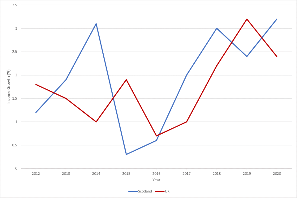
Figure 12 shows a comparison of public sector earnings growth between 2012 and 2020. Scottish public sector earnings growth increases from around 1.2% in 2012 up to 3% in 2014, before falling to less than 0.5% in 2015. There is then a general increase up to 2018, reaching 3% once more before falling in 2019 and increasing again in 2020. UK public sector earnings growth follows a different pattern to Scotland. It begins just below 2% in 2012 and falls gradually to 1% in 2014. There is a rise in 2015, followed by a fall to around 0.75% in 2016. There is increased earnings growth which is generally lower than that of Scotland up to 2019, up to around 3% and falls below Scottish growth in 2020 to around 2.5%.
Changes in public sector pay could explain the divergence. Public sector employment is not directly observable in the data. However, a proxy for the public sector using information on sector is sufficient to test the theory. The following sectors are excluded from the treated and control groups: ‘Public Administration’, ‘Education’, and ‘Human Health’. To confirm confounding by public sector pay, the difference should be closer to zero.
Table 20: Percentage change in income for band 3 excluding the public sector.
| Band Number | Lower Threshold | Upper Threshold | Nearest Neighbour (1) | Nearest Neighbour (2) | Kernel (Epan) |
|---|---|---|---|---|---|
| 3 | £24,001 | £43,430 | -0.00083 | -0.00118* | 0.000105 |
We convert the result in the table above to get the following range of elasticities:
Table 21: TIEs for income band 3 excluding the public sector.
| Band Number | Lower Threshold | Upper Threshold | Nearest Neighbour (1) | Nearest Neighbour (2) | Kernel (Epan) |
|---|---|---|---|---|---|
| 3 | £24,001 | £43,430 | 0.07 | 0.09* | -0.01 |
The elasticities within this income band are much closer to zero, and generally not statistically significant. The test confirms Scottish taxpayer income grew at approximately the same rate as its matched control group in sectors not dominated by the public sector.
We conclude that the difference in public sector pay growth in Scotland confounds the results for Intermediate rate taxpayers. The percentage change in income is now not statistically significantly different from zero, and negative across two of the matching approaches.
These results fit much better with expectations that individuals within this income band have almost no behavioural effects to tax changes. This concurs with Gruber and Saez’s (2002) findings that individuals within a similar sized income band exhibit a small behavioural response. In their paper, they find an elasticity of taxable income between 0.18 and 0.28 for individuals with income between $10,000 and $50,000.
We therefore conclude that after accounting for the change in public sector pay, there is little to no divergence in income growth between the two groups, and by inference no fall in taxable income as a result of the policy across the Starter, Basic and Intermediate rate bands.
13. Conclusion
Our paper has contributed to the literature by providing the first insights into how Scottish taxpayers responded to the five-band policy in 2018 to 2019. We took this unique opportunity to analyse a natural experiment, comparing Scottish taxpayers to a matched control group of similar taxpayers from rUK, where Income Tax rates remained the same.
Overall, our results were broadly consistent with the published literature, providing some limited evidence of Scottish taxpayers lowering their taxable income in response to increasing tax rates. As expected, the size of the behavioural response generally increased with increasing income levels.
Our results were also relatively stable under different methodological approaches. It is worth noting that our study excluded people who moved between Scotland and rUK, so the behaviour covered in our paper only relates to taxpayers who remain where they are and alter the amount of income they declare in response to the policy. It is possible that some taxpayers may instead have moved between Scotland and rUK as a result of the policy.
The behavioural effects were largest for taxpayers earning over the rUK Additional rate and Scottish Top rate threshold of £150,000. Our overall elasticity for these taxpayers was comparable to and somewhat larger than HMRC’s previous 2012 estimate of 0.45, ranging from 0.52 to 0.77 depending on the control group matching methodology used. This result is more in line with estimates produced by IFS researchers (Browne and Phillips, 2017) and Brewer et al. (2010).
Our estimates for each of the three income bands over £150,000 increased with increasing income levels. The results are a little unstable for this group depending on the matching methodology used and this is likely due to the relatively small numbers of taxpayers in these bands. With any analytical study, an estimate based on a small population size can be more susceptible to uncertainty and volatility. Our results are broadly similar to those found in USA studies, and higher than results found in studies from other countries such as Norway and Denmark.
For Scottish individuals with incomes above the 2018 to 2019 Scottish Higher rate threshold of £43,431 and below £150,000, we found evidence of a limited behavioural response, smaller than for those earning more than £150,000. For the most part, the behavioural effects increased with income (aside from an unusually small result for incomes above the Personal Allowance Taper between £123,701 and £150,000).
Our results for Scottish taxpayers within the Scottish Higher rate band were somewhat higher than those anticipated from the published literature on TIEs. Research on TIEs tends to focus more on higher income individuals, as it is often assumed that there will be little or no behaviour at lower income levels. Our results were a little larger than those found in previous studies of behaviour at similar income levels, ranging from 0.12 to 0.46 compared to the 0.11 to 0.27 found by Gruber and Saez (2002).
We initially found some counterintuitive results for Scottish taxpayers with taxable income below £43,431, where they appeared to increase their taxable income relative to similar taxpayers in rUK. However, we found that this was mostly driven by evidence of higher growth in public sector pay in Scotland relative to the UK as a whole. When a proxy for the public sector was excluded, we found much more intuitive results, with little to no evidence of any behavioural effect. This is in line with expectations from the literature.
14. References
Aarbu, K. & Thoresen, T., 2001. Income Responses to Tax Changes - Evidence from the Norwegian Tax Reform. National Tax Journal, 54(2), pp. 319-335.
Abadie, A. & Imbens, G., 2006. Large sample properties of matching estimators for average treatment effects. Econometrica, 74(1), pp. 235-267.
Brewer, M., Saez, E. & Shephard, A., 2010. Means-testing and Tax Rates on Earnings, Oxford: Oxford University Press.
Browne, J. and Phillips, D., 2017. Updating and critiquing HMRC’s analysis of the UK’s 50% top marginal tax rate. [Online] Available at: https://ifs.org.uk/publications/9677.
Companies House, 2018. Standard industrial classification of economic activities (SIC). [Online] Available at: https://www.gov.uk/government/publications/standard-industrial-classification-of-economic-activities-sic.
Feldstein, M., 1995. The Effect of Marginal Tax Rates on Taxable Income: A Panel Study of the 1986 Tax Reform Act. Journal of Political Economy, 103(3), pp. 551-572.
Gruber, J. & Saez, E., 2002. The elasticity of taxable income: evidence and implications. Journal of Public Economics, Volume 84, pp. 1-32.
Heckman, J., Ichimura, H. & Todd, P., 1997. Matching as an econometric evaluation estimator: evidence from evaluating a job training programme. Review of Economic Studies, 64(4), pp. 605-654.
HMRC, 2012. The Exchequer effect of the 50 per cent additional rate of income tax, HM Revenue & Customs.
Jann, B., 2017. kmatch: Kernel matching with automatic bandwidth selection. [Online] Available at: http://repec.org/usug2017/jann-uksug17.pdf.
Kleven, H. J. & Schultz, E. A., 2014. Estimating Taxable Income Responses Using Danish Tax Reforms. American Economic Journal: Economic Policy, 6(4), pp. 271-301.
Lenhart, O., 2019. The effects of health shocks on labor market outcomes: evidence from UK panel data. The European Journal of Health Economics, Volume 20, pp. 83-98.
Lindsey, L., 1987. Individual Taxpayer Response to Tax Cuts: 1982-1984 With Implications for the Revenue Maximizing Tax Rate. Journal of Public Economics, Volume 33, pp. 173-206.
ONS, 2021. HI00 Regional labour market: Headline Labour Force Survey indicators for all regions. [Online] Available at: https://www.ons.gov.uk/employmentandlabourmarket/peopleinwork/employmentandemployeetypes/datasets/headlinelabourforcesurveyindicatorsforallregionshi00/current.
ONS, 2021. Regional gross domestic product: all ITL regions. [Online] Available at: https://www.ons.gov.uk/economy/grossdomesticproductgdp/datasets/regionalgrossdomesticproductallnutslevelregions.
Rosenbaum, P. R. & Rubin, D. B., 1983. The central role of the propensity score in observational studies for causal effects. Biometrika, 70(1), pp. 41-55.
Saez, E., 2004. Reported Incomes and Marginal Tax Rates, 1960-2000: Evidence and Policy Implications. In: J. M. Poterba, ed. Tax Policy and the Economy, Volume 18. National Bureau of Economic Research, pp. 117-174.
Saez, E., Slemrod, J. & Giertz, S. H., 2012. The Elasticity of Taxable Income with Respect to Marginal Tax Rates: A Critical Review. Journal of Economic Literature, 50(1), pp. 3-50.
Scottish Fiscal Commission, 2021. How we forecast income tax. [Online] Available at: https://www.fiscalcommission.scot/wp-content/uploads/2021/05/How-we-forecast-income-tax-May-2021.pdf.
Scottish Government, 2020. Annual survey of hours and earnings: 2020. [Online] Available at: https://www.gov.scot/publications/annual-survey-of-hours-and-earnings-2020/.
15. Annexes
15.1 Annex A – Information on population included within Results Section
The information within Table A1 shows figures for the number of treated and untreated individuals used within the propensity score matching approach. These apply for the nearest neighbour matching approaches.
Table A1: Number of individuals in each income band, treated and untreated for nearest neighbour matching.
| Income Band | Income Range | Number Treated on Support | Number Untreated on Support | Number of observations |
|---|---|---|---|---|
| Band 10 | £500,000 + | 1,077 | 39,546 | 40,623 |
| Band 9 | £300,001 - £500,000 | 1,761 | 50,255 | 52,016 |
| Band 8 | £150,001 - £300,000 | 10,524 | 210,524 | 221,048 |
| Band 7 | £123,701 - £150,000 | 8,327 | 129,203 | 137,530 |
| Band 6 | £100,000 - £123,700 | 14,982 | 216,813 | 231,795 |
| Band 5 | £80,001 - £100,000 | 24,270 | 337,392 | 361,662 |
| Band 4 | £43,431 - £80,000 | 216,029 | 2,681,890 | 2,897,919 |
| Band 3 | £24,001 - £43,430 | 757,065 | 8,044,788 | 8,801,853 |
| Band 2 | £13,851 - £24,000 | 856,427 | 9,274,384 | 10,130,811 |
| Band 1 | £11,850 - £13,850 | 182,859 | 2,070,757 | 2,253,616 |
15.2 Annex B
The figures below show the propensity scores before and after matching for each income band with nearest neighbour one-to-one matching. On the left, the graph shows the density of propensity scores for the treated and control groups before matching, where we generally see that there are sizeable differences in the density of propensity scores. On the right we see significant overlap between the treated and matched control groups.
Figure A1: Band 1.
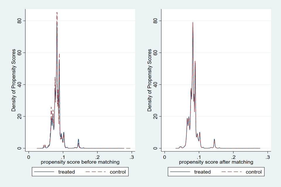
Figure A2: Band 2.
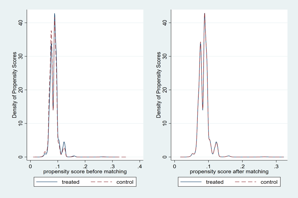
Figure A3: Band 3.
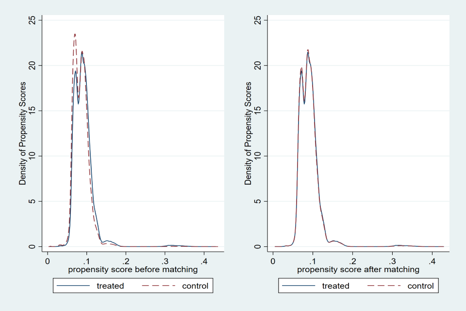
Figure A4: Band 4.
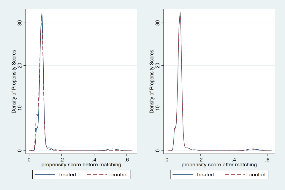
Figure A5: Band 5.
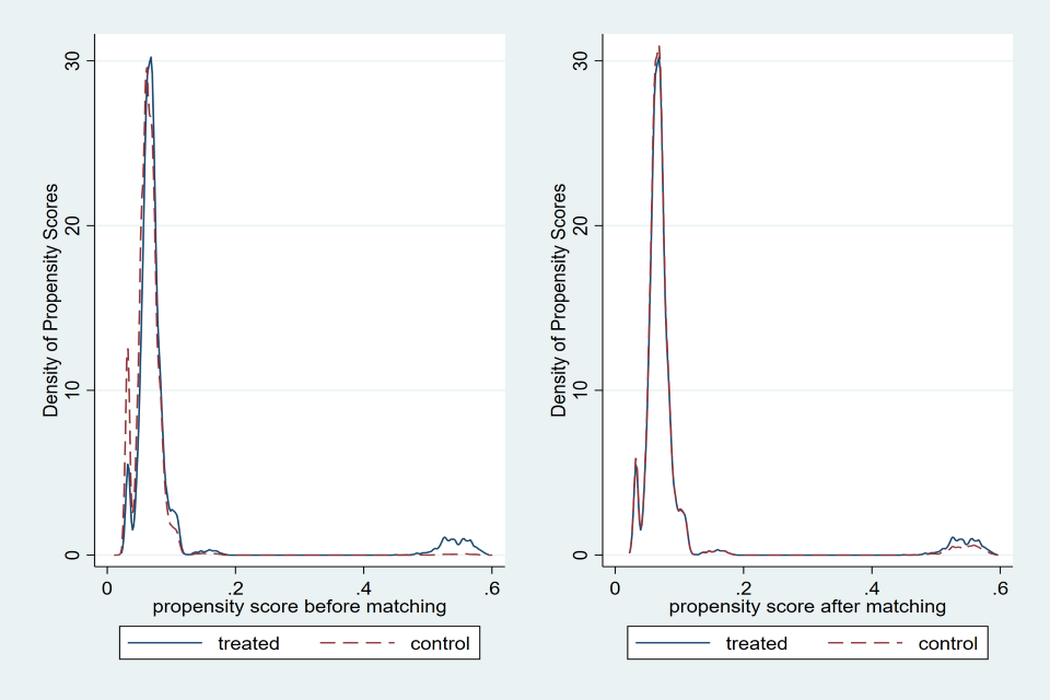
Figure A6: Band 6.
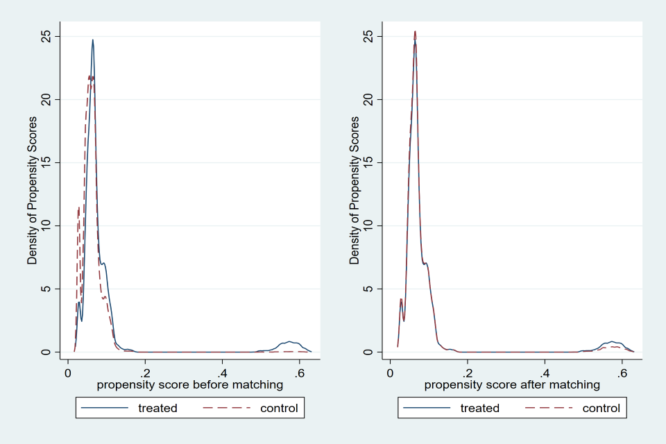
Figure A7: Band 7.
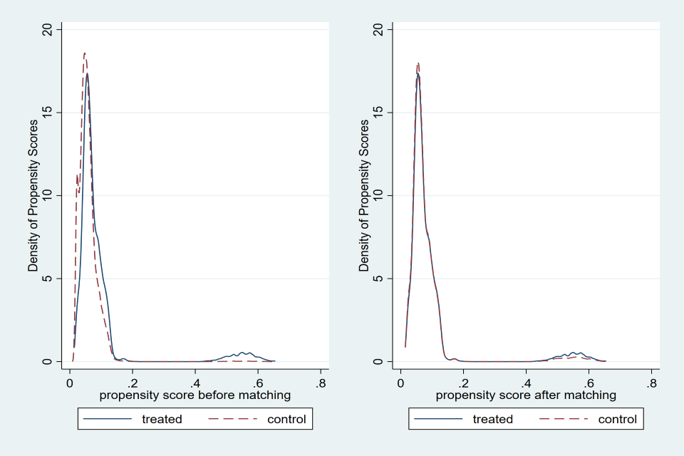
Figure A8: Band 8.
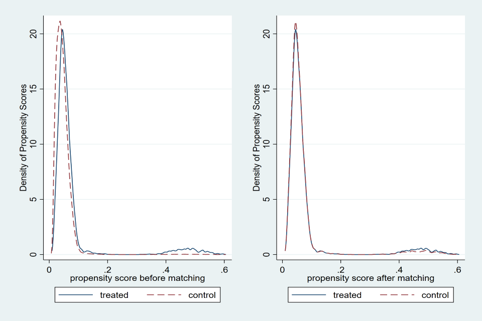
Figure A9: Band 9.
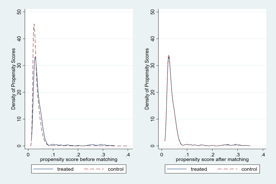
Figure A10: Band 10.

15.3 Annex C – Alternative Specifications
This section presents alternative methods of matching and estimating propensity scores as a robustness check to the main research design. Column three shows the nearest neighbour with replacement using a probit model to estimate propensity scores. Column four shows the nearest neighbour without replacement using a logit model to estimate propensity scores.
Table A2: Results from alternative specifications.
| Income Band | Income Range | Probit, 1 Nearest Neighbour, with replacement | Logit, 1 Nearest Neighbour, without replacement |
|---|---|---|---|
| Band 1 | £11,850 - £13,850 | 0.00104, (0.00166) | -0.000341, (0.00159) |
| Band 2 | £13,851 - £24,000 | 0.00401***, (0.000644) | 0.00458***, (0.000618) |
| Band 3 | £24,001 - £43,430 | 0.00294***, (0.000594) | 0.00272***, (0.000562) |
| Band 4 | £43,431 - £80,000 | -0.00265**, (0.00125) | -0.00504**, (0.00119) |
| Band 5 | £80,001 - £100,000 | -0.00599, (0.00469) | -0.00583, (0.00437) |
| Band 6 | £100,000 - £123,700 | -0.00985, (0.00660) | -0.136**, (0.00625) |
| Band 7 | £123,701 - £150,000 | -0.00125, (0.00927) | 0.000760, (0.00889) |
| Band 8 | £150,001 - £300,000 | -0.00555, (0.00937) | -0.00931, (0.00888) |
| Band 9 | £300,001 - £500,000 | -0.0135, (0.0280) | -0.0429, (0.0263) |
| Band 10 | £500,000 + | -0.0511, (0.0418) | -0.0959*, (0.0421) |
Standard errors in parentheses. *** p < 0.01, ** p<0.05, * p<0.1
15.4 Annex D – Removing the Public Sector from Band 2 and Band 3
Table A3: Percentage change in income excluding the public sector.
| Income Band | Income Range | 1 Nearest Neighbour | 2 Nearest Neighbours | Kernel |
|---|---|---|---|---|
| Band 2 | £13,851 - £24,000 | 0.00214***, (0.000782) | 0.00237***, (0.000673) | 0.00269***, (0.000689) |
| Band 3 | £24,001 - £43,430 | -0.000826, (0.000758) | -0.00118*, (0.000655) | 0.000105, (0.000693) |
Standard errors in parentheses. *** p < 0.01, ** p<0.05, * p<0.1