Research and analysis

Youth Employment Initiative – Impact Evaluation Technical Annex

Published 2 March 2022

Introduction

This technical annex provides additional detail on the impact evaluation of the Youth Employment Initiative (YEI). The results from the impact evaluation and a top-level summary of the methodology employed, including the rationale, are provided in the main report. The technical annex covers and is structured as follows:

1. Constructing the evaluation dataset. This chapter covers the variables used in the analysis, how the treatment group and comparator pool (i.e. a sample from the wider population) were identified in administrative data, and the linking of the various datasets to produce an evaluation dataset for analysis.

2. The analytical procedure: This chapter covers the assignment of pseudo-start dates (to the comparator group), calculating pre- and post- intervention employment/benefit periods, selecting the analysis cohort, and details of the propensity score matching undertaken.

1. Constructing the evaluation dataset

The impact evaluation of the Youth Employment Initiative drew on data from a range of sources and was subject to transformations prior to analysis. This chapter provides detail on the variables used in the analysis, and how these were linked and transformed to construct the evaluation dataset.

1.1. Data sources and variables

Table 1.1 details the data sources, variable names and the codes used in the analysis. All variables in the table below were collected for both treatment and comparator pool groups, except for variables from the ‘ESF Evaluation Created’ and ‘ESF management information sources’ rows as they were used to identify the treatment group.

Table 1.1: Data source and variables

Source	Variable name	Variable code
ESF Evaluation Created	Participant No	Participant_ID_Ecorys
	Group	Group
	Duplicate ID	Duplicate_YEI_individual
(DWP) Customer Information System	Date of Birth	CIS_DoB
	Gender	CIS_Sex
	Local authority	LA_Name
Index of multiple deprivation data (linked by LSOA)	IDACI Score	IDACI
	IMD Score	IMD
ESF management information	Flag if on other ESF	Other_ESF_YEI_Flag
	Provider ID or Provider Name	Project_name
	YEI Provision Start Date	Date_of_entry_clean
YEI Provision End Date	Date_of_leaving_clean
Employment Status on Leaving	emp_status_on_leaving_clean
Education or Training on Leaving	ed_or_train_on_leaving_clean
HMRC - Real Time Information (RTI)	Payroll spell start date	payrollspellstart
	Payroll spell end date	payrollspellend
Payroll spell pay amount (sum)	payrollspellpay
DWP National Benefits Database	Disability Living Allowance Spell Start Date	DLAspellstart
	Disability Living Allowance Spell End Date	DLAspellend
	Employment and Support Allowance Spell Start Date	ESAspellstart
	Employment and Support Allowance Spell End Date	ESAspellend
	Incapacity Benefit Spell Start Date	IBspellstart
	Incapacity Benefit Spell End Date	IBspellend
	Carers Allowance Spell Start Date	ICAspellstart
	Carers Allowance Spell End Date	ICAspellend
	Income Support Spell Start Date	ISspellstart
	Income Support Spell End Date	ISspellend
	Jobseekers Allowance Spell Start Date	JSAspellstart
	Jobseekers Allowance Spell End Date	JSAspellend
	Passported Incapacity Benefit Spell Start Date	PIBspellstart
	Passported Incapacity Benefit Spell End Date	PIBspellend
Personal Independence Payment Datasets	Personal Independence Payment Spell Start Date	PIPspellstart
	Personal Independence Payment Spell End Date	PIPspellend
UC Full Service, UC Live Service	Universal Credit Spell Start Date	UCspellstart
	Universal Credit Spell End Date	UCspellend

Notable variables not included in the analysis and the reasons why were as follows:

• A range of educational background and qualification variables were requested from the Department for Education to be linked to the YEI treatment and comparator groups through the Longitudinal Educational Outcomes (LEO) project. Variables included educational achievement, attendance and exclusions, as well as background characteristics such as ethnicity. This data was unavailable within the evaluation timescales. This led to an adaptation of the CIE design, which is detailed in Section 2.3.
• Owing to incomparable or missing data across different types of benefits, destination codes were not included. For example, destination codes for Job Seekers Allowance were available but there is no equivalent for Universal Credit.
• Ethnicity was requested and received from DWP. However, owing to high levels of missing data for the comparator pool, ethnicity was not included in the final analysis.
• Data for self-employment was not available.

1.2. Constructing the treatment group and comparator pool

Prior to the impact analysis (detailed in Chapter 2), it was necessary to identify individuals that:

• Were supported by YEI and could be linked to the administrative datasets detailed in Section 1.1. This was the treatment group.
• Were not supported by YEI (or other ESF provision) and identifiable in administrative datasets. This was the comparator pool from which the analysis draws a final comparator group (i.e. a subset) from.

The process to construct the treatment group and comparator pool are discussed in turn below.

1.2.1. The treatment group

The treatment group was identified through the following steps:

• YEI providers submitted participant IDs, management information and contact details of supported individuals to DWP.
• DWP fuzzy matched supported individuals, using contact details, to the Customer Information System (CIS). Without unique identifiers such as National Insurance Numbers (NINos) exact matching on contact details would have yielded few matches. Therefore, to ensure a greater match rate Fuzzy matching was employed as it identifies similar records to one another and matches those falling within a set parameter. This approach ensures small variations in contact details (between YEI provider submitted and CIS) did not prevent individuals being matched. The CIS contained National Insurance Numbers (NINos) that enable linking to the administrative datasets detailed in Section 1.1.
• DWP cleaned the treatment group to only include individuals who were within the YEI age criteria (15-29) and were not in employment or education/training when they started support.

The resulting treatment group comprised 3,276 individuals. This is much fewer than the number actually supported by YEI. The main reason for this was missing contact details from YEI providers. A smaller proportion had contact details but could not be matched.

At the time the treatment group was created in March 2019, labour market status for those participants who could be matched to CIS was very similar to the overall YEI population. Table 1.2 provides a comparison between those able to be matched to CIS at the point the treatment group was created and the overall population of YEI participants at that point. Relative to the total YEI population, a slightly higher proportion of those that could be matched to CIS were long term unemployed, while a slightly lower proportion were unemployed. The data indicates that the labour market status of the treatment group, in terms of the balance between long-term unemployment, unemployment and inactivity, closely reflects that of all participants on the programme.

Table 1.3: Comparison of YEI participants that could be matched to CIS and all YEI participants at March 2019

Labour market status	CIS match possible	Total YEI population
Long Term Unemployed	32.87%	30.89%
Unemployed	39.47%	42.25%
Inactive – in education	0.17%	0.15%
Inactive Not in education or training	27.50%	26.71%

1.2.2. The comparator pool

To maximise the likelihood of identifying a well-matched comparison group, a stratified sample was drawn from CIS (and subsequently linked to administrative datasets). Based on analysis of the YEI treatment group, the comparator pool consisted of 50,000 individuals from the general population (i.e. all those on CIS) and a further 50,000 that are known to have claimed out of work benefits^{[footnote 1]}. Both the general population and out of work benefit groups were then sampled based on age and gender (Table 1.3).

Table 1.3: Comparator pool stratification

Age group	Proportion of sample	Est. number in comparator pool(n=100,000) – Total	Est. number in comparator pool(n=100,000) – Male 58%	Est. number in comparator pool(n=100,000) – Female 42%
16 - 19	47%	47,000	27,260	19,740
20 - 24	37%	37,000	21,460	15,540
25 - 29	16%	16,000	9,280	6,720
Total	100%	100,000	58,000	42,000

The comparator pool was cleaned to, as far as possible, removing individuals who had been supported by YEI and/or other ESF provision, in the current funding period. Following the cleaning, the comparator pool comprised 97,444 individuals. The cleaning relied on individuals being identifiable in the CIS using YEI/ESF provider submitted data and DWP held management information. As such, it is possible that some individuals who did receive YEI/ESF support but could not be linked to the CIS, appear in the comparator pool. Whilst all practical steps were taken to minimise this, it is possible there was some contamination of the comparator pool.

1.3. Preparing the evaluation dataset

Following the identification of the treatment group and comparator pool in CIS, records were matched (using NINos) to the key datatsets required for background characteristics and outcomes. The datasets included:

• HMRC - Real Time Information (RTI)
• DWP National Benefits Database
• Personal Independence Payment Datasets
• UC Full Service, UC Live Service

The specific variables from each are detailed in Table 1.1. Prior to the data being shared with Ecorys, DWP undertook cleaning of the raw data to account for overlapping employment spells (with the same employer) and benefit claims, and current/ongoing employment spells and benefit claims. For all datasets, the cleaning was conducted in line with the respective data owners’ procedures (or where these weren’t formally in place, in consultation with them).

The resulting evaluation dataset comprised a single row for each individual in the treatment group or comparator pool and separate columns for each distinct employment spell (i.e. with a different employer) and/or benefit claim.

All data was pseudo-anonymised prior to being shared with Ecorys.

2. Analytical procedure

Drawing on the evaluation dataset provided by DWP, additional variable transformations, primarily calculating employment/benefit spells pre- and post- YEI, and analysis were undertaken. This chapter provides detail (additional to that provided in the main report) on the analytical procedures followed.

2.1. Assigning pseudo start dates

To reflect that labour market conditions, and thus employment outcomes, vary over time, pseudo start dates were assigned to individuals in the comparator pool. The comparator pool comprises all non-treated (i.e. non-YEI) individuals prior to any matching. Pseudo start dates had to be applied prior to matching so that pre-intervention employment/benefit histories could be constructed (and subsequently used in the matching process). Pseudo start dates were generated to mirror the distribution of start dates for the treatment group and then allocated at random to individuals in the comparator pool.

Pseudo leaving dates were also calculated based on the average duration of YEI interventions (c. 80 days). This enabled analysis of outcomes after leaving the intervention for both the treatment and comparator group.

To test the sensitivity of the analysis to the assignment of pseudo start dates, analysis was run with pseudo start dates mirroring the treatment group but allocated using different random seeds, and with pseudo start dates generated and assigned randomly (ignoring the distribution of start dates for the treatment group). The impact results from these tests did not change substantially.

2.2. Calculating employment and benefit spells

To calculate pre-intervention background characteristics (e.g. pre-intervention employment spells) and relevant outcome measures for the treatment group and comparator pool, the following time intervals were created:

• Pre-YEI: any time before the intervention start date
• 6 months pre-YEI: the 6 months immediately before the intervention start date
• 12 to 6 months pre-YEI: the 6 months prior to the above. (see Section 2.3 for rationale)
• Post-YEI: any time after the intervention leaving date
• 6 months post-YEI: the 6 months immediately after the intervention leaving date

Payment and/or benefit spells in the data were then overlaid on these intervals so that the number of days falling into each could be calculated. Figure 2.1 below illustrates the different intervals:

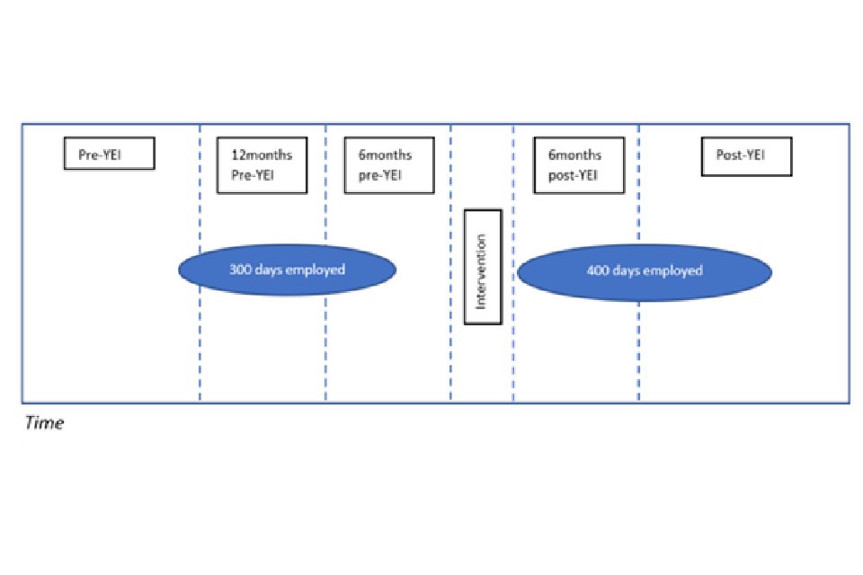
Figure 2.1: Illustration of employment/benefit spell intervals

In the simplified example in Figure 2.1, the blue ovals represent employment spells (these could also be spells on different types of benefits). The number of days falling into each interval are then calculated. In this example, prior to the intervention approximately 100 (of the 300 days overall) were in the 6 month pre-YEI interval. Most of the remaining days for the same employment spell fall into the 12-6 months pre-YEI interval. Post intervention, there was a new employment spell of 400 days, of which, 180 days are in the 6 month interval immediately after the intervention (i.e. the individual was employed for the whole 6 months).

The rationale for setting up the data using this approach is:

• The requirement for comparable pre and post intervals to assess changes in outcomes. As described in the next section, having the data in this format allowed the analysis to focus on individuals who were, theoretically, available for work for the 6 months prior to intervention – hence they could be compared fairly to post intervention periods.
• It accounted for the number of days falling into different intervals: for example, was an individual out of work for all of the 6 months before the intervention, or just a few weeks? Understanding an individual’s engagement with the labour market (through employment and out of work benefits) at different periods can be considered a proxy for their motivation to work.

2.3. Selecting the analysis cohort

As mentioned in the previous section, it was important to ensure that fair pre and post comparisons around outcomes could be made. Based on the data available and programme design, the key outcome of interest was the number/proportion of days worked in the 6 months post YEI, relative to the 6 months pre YEI. However, this outcome only holds if there is confidence that an individual was available for work in the 6 months prior to intervention. If, for example, an individual was in full time education during this pre-YEI period, it would be inappropriate to compare this against a post-YEI period where they had finished education (and were actually available for work). To mitigate this risk, as far as possible with the available data, the following rules/criteria were developed:

1. In the 12 to 6 months prior to the intervention (the second segment of Figure 2.1), the individual had an employment spell of at least 30 days (indicating they were engaged with labour market and likely to be available for work in the 6 months immediately before the intervention). AND, in the 6 months immediately before the intervention (the third segment of the diagram), there was a gap in employment spells of at least 30 days (indicating they were out of work for a period and eligible for support).

2. For the JSA group, in the 12 to 6 months prior to the intervention, the individual had a JSA benefit spell of at least 30 days (indicating they were looking for work and likely to be available for work in the 6 months immediately before the intervention). AND, in the 6 months immediately before the intervention, there was also a JSA benefit spell of at least 30 days (indicating they were out of work and eligible for support).

3. For the ESA group, in the 12 to 6 months prior to the intervention, the individual had an ESA benefit spell of at least 30 days (indicating they were looking for work and likely available for work in the 6 months immediately before the intervention). AND, in the 6 months immediately before the intervention, there was also an ESA benefit spell of at least 30 days (indicating they were likely to be out of work and eligible for support).

If an individual in the treatment group or comparator pool met any of these criteria, they were retained for analysis.

Focusing on this cohort led to a reduction in the treatment group size (from 3,276 to 1,050). In the absence of educational datasets, which could have confirmed whether an individual was in full time education prior to YEI (and be accounted for in the analysis) and their progression after the intervention, this was a necessary step.

2.4. Propensity score matching

A hybrid nearest neighbour and exact matching approach was implemented on the analysis cohort detailed in the previous section. The following variables were used for matching:

• Age on start of YEI:
• (binary) Sex
• Month of YEI start
• Year of YEI start
• Index of Multiple Deprivation (IMD) score for home address (Lower Layer Super Output Area or LSOA)
• Region (of home address)
• Total number of days in employment pre-YEI
• Number of days in employment in the 6 months pre-YEI
• Total number of days on JSA pre-YEI
• Number of days on JSA in the 6 months pre-YEI
• Total number of days on ESA pre-YEI
• Number of days on ESA in the 6 months pre-YEI
• Total number of days on UC pre-YEI
• Number of days on UC in the 6 months pre-YEI
• Total number of days on IS pre-YEI
• Number of days on IS in the 6 months pre-YEI
• (binary) claiming disability related benefits pre-YEI
• (binary) claiming carer benefits pre-YEI
• (binary) meets criteria 1 (see previous section)
• (binary) meets criteria 2 (see previous section)
• (binary) meets criteria 3 (see previous section)

To ensure fair comparisons (detailed in previous section) the final 3 variables in the list above and year of YEI start were specified in the matching algorithm as “exact”. This meant that any potential comparator case could only match with a treated case if there was an exact match on these variables. For example, only those in the comparator group meeting the JSA rule (criteria 2) could be matched to treated cases meeting the same criteria.

Up to 3 matches per treated case were allowed. Cases not meeting the common support rule were discarded and a caliper setting of 0.1 was used.

Following the matching procedure, standardised mean differences between the treatment and comparison group were calculated and are detailed in Table 2.1. A high level of balance was achieved. All variables were below the DWP threshold for standardised mean differences of 0.05, other than month of YEI start (‘Month_Entry’ in Table 2.1, which showed a standardised mean difference of 0.0518). Furthermore, the vast majority (495 of 576) of all two-way interactions of the variables were below the 0.05 threshold. The interactions outside of this threshold were below or just above the less stringent but widely accepted threshold of 0.1. Additional analysis of the distributions of continuous variables was undertaken, which further confirmed good balance had been achieved.

Table 2.1: Standardised mean differences between treatment and comparator groups

Variable	Variable type	Mean standardised difference	Balanced (at <0.05 threshold)
Distance	Distance	0.0088	Balanced
Age	Contin.	-0.0106	Balanced
CIS_Sex_M	Binary	0.0155	Balanced
Month_entry	Contin.	0.0518	Not Balanced
Year_entry	Contin.	0	Balanced
IMD	Contin.	-0.0129	Balanced
Region_East Midlands	Binary	-0.0177	Balanced
Region_East of England	Binary	-0.0003	Balanced
Region_London Binary	0.0028	Balanced
Region_North East	Binary	-0.0047	Balanced
Region_North West	Binary	0.0064	Balanced
Region_South East	Binary	-0.0017	Balanced
Region_South West	Binary	-0.0007	Balanced
Region_West Midlands	Binary	0.0191	Balanced
Region_Yorkshire and The Humber	Binary	-0.0031	Balanced
Pre_yei_employment_days	Contin.	0.0017	Balanced
Pre_yei_employment_days_6	Contin.	0.006	Balanced
Pre_yei_jsa_days	Contin.	0.0142	Balanced
Pre_yei_jsa_days_6	Contin.	0.0003	Balanced
Pre_yei_esa_days	Contin.	0.0207	Balanced
Pre_yei_esa_days_6	Contin.	0.0036	Balanced
Pre_yei_uc_days	Contin.	0.0233	Balanced
Pre_yei_uc_days_6	Contin.	-0.0008	Balanced
Pre_yei_is_days	Contin.	-0.0031	Balanced
Pre_yei_is_days_6	Contin.	-0.0112	Balanced
Disabled	Binary	0.0045	Balanced
Carer	Binary	-0.0031	Balanced
Emp_criteria	Binary	0	Balanced
Jsa_criteria	Binary	0	Balanced
Esa_criteria	Binary	0	Balanced

1. Included individuals that claimed out of work benefits at any time between 1st January 2016 and 18th December 2017 ↩