Research and analysis

Annexe 5

Published 28 July 2020

RQV. What is the relationship between the Value of a Life Year and the Value of a Prevented Fatality?

1. Introduction

1.1. Background and Coverage of this Chapter

In this research question (RQ), we begin with a formal specification of a Value of Life Year (VOLY) and follow this with the framework used to derive a VOLY indirectly from an existing Value of a Prevented Fatality (VPF). This allows us to set out the theoretical underpinnings of the relationship between the (value of) prevening fatalities and a (value of) statistical life year(s) in the most commonly applied VOLY estimation framework to date. Whilst this cannot directly address the issue of when it is more appropriate to use the VPF over the VOLY (or vice versa), a clear understanding of the 2 frameworks can assist in the judgements that must necessarily be made should mortality risk valuation for regulatory analysis evolve in this way in the future. However, as noted in Schedule A, the use of both a constant VPF and a constant VOLY can be seen to be at variance with each other, since the latter implies, for consistency, the application of an age-dependant VPF in policy^{[footnote 1]}. We also introduce a number of potential methods to empirically estimate a VOLY based on developing or adapting procedures already suggested or deployed in the field. We comment primarily on their potential to be taken forward to an empirical study and leave until the final report a consideration of how, if at all, any resulting empirical data then might be harnessed to contribute to answering what, in this case, is a largely conceptual question i.e. the relationship between the 2 measures.

In the second part (section 5), we draw on evidence currently available in the mortality risk valuation literature to explore some factors identified in Schedule A by the contractor that might inform or affect the relationship between the VPF and VOLY, specifically: health perceptions throughout the lifecourse; personal time preference rates; whether the value of life year might be expected to decline as the (gain in) life expectacy increases; whether changes in the utility opportunity cost of money may occur as a person ages and the implication of this for the value of a life expectancy gain; other age-related impacts; and, finally, whether, from a behavioural perspective, there might be some inherent disutility of a sudden, possibly untimely, death in the next period relative to death in the future, particularly if the primary impact of reducing that risk is viewed as a change in life expectancy.

This RQ is framed around answering the specific questions identified in Schedule A. We applied a pragmatic literature search strategy. In doing so, we use, where appropriate, specific papers or reports to guide the initial response, supplemented by, where available, (sometimes limited) evidence from the wider literature. In addition, given the natural overlap of at least some of these issues with other RQs, the reader is pointed to those RQs for further discussion.

2. The VPF and the VOLY

We begin with a formal specification of a VOLY and follow this with the framework used to derive a VOLY indirectly from an existing VPF^{[footnote 2]}. We first set out some basic concepts and definitions. Then, prior to considering the potential for direct empirical elicitation of a VOLY, we clarify a potential problem with a commonly adopted conceptual approach. This approach is to conceive the VPF as a sum of constant VOLYs, discounted at some chosen rate, for example the social rate of time preference in the UK (1.5%). This assumption underpins – either explicitly or implicitly – previous attempts to derive a VOLY from the VPF – and we attempt to clarify why this is inappropriate in all but one circumstance.

2.1. Basic concepts and definitions underpinning a VOLY

With time, t, measured in years from the present (so that t = 1 denotes the coming year, t = 2 the year after that and so on), an individual’s “hazard rate”, p_t, for year t is the probability that the individual will die during that year, conditional on surviving to the beginning of the year. Assuming for the sake of simplicity that if death is to occur in year t then it does so at the beginning of the year, it then follows that viewed from the present, the individual’s probability of surviving year 1 is (1 - p₁), the probability of surviving year 2 is (1 - p₁)(1 - p₂), the probability of surviving year 3 is (1 - p₁)(1 - p₂)(1- p₃) etc. The individual’s remaining life-expectancy, E, is therefore, by definition^{[footnote 3]}, given by:

Equation 1

E = (1 - p₁) + (1 - p₁)(1 - p₂) + (1 - p₁)(1 - p₂)(1 - p₃) + . . .

It therefore follows that, given the definition of remaining life-expectancy, the only way in which remaining life expectancy can be increased is by reducing the hazard rate in the coming year or in some future year or years. For illustrative purposes, let us focus on a gain in life-expectancy generated by a reduction in the hazard rate for the coming year. From equation (1) it follows that:

Equation 2

The gain in life-expectancy, δE, resulting from a marginal reduction, δp₁ , in p₁ is therefore given by:

Equation 3

δE = E δp₁ / (1 - p₁)

so that with p₁ small (as will typically be the case for anyone below the age of 80), to a close approximation, δE will be given by:

Equation 4

δE = E δp₁ .

Now consider a large group of individuals each enjoying a marginal gain in life-expectancy resulting from a reduction in their hazard rate for the coming year where, taken across the affected group, these marginal gains in life expectancy sum to one year. This can therefore naturally be referred to as a gain of one “statistical life year”. Summed across the affected group of individuals, total willingness-to-pay (WTP) for the marginal hazard rate reductions that generate the gain of one statistical life year can therefore naturally be regarded as the WTP – based value of a statistical life year (VOLY) for the group concerned.^{[footnote 4]}

2.2. Deriving the VOLY from a pre-determined Value of Preventing a Statistical Fatality (VPF)

Consider a large group of n individuals each enjoying a 1/n marginal reduction in the hazard rate for the coming year, thereby preventing one statistical fatality. Summed over the affected group, aggregate WTP for these marginal risk reductions therefore constitutes the WTP-based Value of Preventing a Statistical Fatality (VPF) for the group concerned. In turn, from equation (4) in the argument developed above, the marginal gain in remaining life-expectancy for the i^th individual resulting from the 1/n marginal reduction in his/her hazard rate for the coming year will be given by E_i/n where E_i is the individual’s current remaining life-expectancy. Summed over the affected group of n individuals, the aggregate gain in life-expectancy is therefore equal to Σ E_i/n = (1 / n)Σ E_i which is, by definition, the mean remaining life-expectancy for individuals in the group. Aggregate WTP for each year of aggregate gain in life-expectancy – which, as already noted, can naturally be regarded as the value of a statistical life year (i.e. the VOLY) – is therefore given by the VPF for the affected group divided by mean remaining life expectancy for the group. Given that the VPF for the affected group is, by the standard argument, equal to the mean marginal rate of substitution, mi , of the i^th individual’s wealth for his/her risk of death during the coming year, in this case the VOLY is therefore equal to the mean of mi divided by the mean of E_i for the affected group.

It should, however, be noted that the VOLY derived by this procedure applies to the gain of a statistical life year generated by:

• individual marginal hazard rate reductions that apply only to hazard rates for the coming year
• marginal hazard rate reductions that are equal across all affected individuals

Now suppose that we retain the assumption that the marginal risk reductions apply only to hazard rates for the coming year, but assume instead that these risk reductions, δp_i, are allowed to vary across the affected group and are set so as to ensure that all of the n affected individuals enjoy the same marginal gain, 1/n, in life expectancy so that, for all i, E_i δp_i = 1/n and hence δp_i = 1/nE_i. It then follows that, summed over the n affected individuals, the aggregate gain in life expectancy will be equal to one year and aggregate WTP will be equal to Σm_i/nE_i = (1/n)Σm_i/E_i. In this case, the aggregate WTP or an aggregate gain of one year of life expectancy (i.e. the VOLY) will therefore be equal to the mean of the ratio, m_i/E_i, rather than, as in the previous case, the mean of m_i divided by the mean of E_i. Clearly, the magnitude of the mean of m_i/E_i relative to the magnitude of the ratio of the means of m_i and E_i will depend on the covariance between m_i and E_i, with the 2 being approximately equal only if m_i and E_i are positively correlated. In fact, empirical evidence indicates that the relationship between m_i and age tends to follow an inverted-U form, peaking in middle age, so that m_i and E_i an reasonably be taken to be positively correlated, at least over the majority of adult years (i.e. from middle age onwards). It therefore seems reasonable to assume that the VOLY derived from the mean of ratios will not differ greatly from the figure derived from the ratio of means.

The argument just developed has, of course, focused on gains in undiscounted life expectancy, but it is clear that with life expectancy defined on a discounted basis precisely the same argument would apply with remaining life expectancy, E_i, replaced by discounted remaining life expectancy, Ed_i.

Up to this point, it is also clear that the argument has focused on gains in life-expectancy generated by marginal reductions that apply only to the hazard rate for the coming year. However, many safety improvements and medical treatments can be expected to provide either a constant ongoing hazard rate reduction over several future years, or – particularly in the case of a reduction in air pollution – a proportional reduction over remaining lifetime which, given that an individual’s hazard rates can be taken to grow at an approximately exponential rate with age, means that the affected individual’s hazard rate reductions will themselves grow exponentially over time. The question is then how the WTP-based value per statistical year’s gain in remaining life-expectancy generated by such ongoing hazard rate reductions can be expected to relate to the value derived for a year’s gain in remaining life-expectancy generated by a reduction in the coming year’s hazard rate. Assuming that the typical individual will effectively apply a positive personal discount rate to anticipated future utilities, then, from a purely theoretical point of view, it would appear that since a gain in life-expectancy generated by a delayed hazard rate reduction will yield a smaller gain in discounted expected utility than the same gain in life-expectancy generated by an earlier hazard rate reduction, then the VOLY applicable to the former will be less than the figure applicable to the latter.

It is also worth noting that since the hazard rate grows at what is effectively an exponential rate with age, then it follows that a proportional reduction in an individual’s future hazard rates will have the same effect on his/her remaining life-expectancy as a reduction in his/her age. As argued in Mason et al. (2009), the individual’s WTP for the resultant gain in life-expectancy will therefore reflect the extent to which his/her remaining lifetime expected utility varies with age and this will, in turn, reflect the way in which the VPF for a group of similar individuals varies with age. Taken across a large group of individuals, aggregate WTP for proportional reductions in future hazard rates that generate marginal gains in life-expectancy which sum to one statistical life year will therefore correspond to the rate at which the VPF for the group varies with age and hence the rate at which it increases with remaining life-expectancy.

Thus, rather than estimating the VOLY as the VPF divided by mean remaining life-expectancy (as would be appropriate if the hazard rate reduction applied only to the coming year), the VOLY for a proportionate reduction in all future hazard rates would be given by the arithmetic mean of the rate at which the VPF for the group affected increases with remaining life-expectancy, with the latter measured in years. More specifically, if the VPF is an increasing function, VPF = f(E), of remaining years, E, of life-expectancy then the VOLY would be given by the arithmetic mean of the derivative, df(E)/dE, taken across the affected group. Since at least some empirical evidence indicates that, at least beyond middle-age, the VPF is an increasing, strictly-concave function of undiscounted life-expectancy – see, for example, Jones-Lee et al. (1985) – it follows that the VOLY estimated as the mean of the derivative df(E)/dE will necessarily be less than the figure obtained by taking the mean of the ratio, VPF/E, which, as argued above, would be the appropriate measure of the VOLY for gains in life-expectancy resulting from hazard rate reductions that apply only to the coming year and afford all affected individuals the same marginal gain in life-expectancy. It should also be noted that given the strict concavity of the function, f(E), both of these VOLY measures will be decreasing functions of remaining life-expectancy and hence increasing functions of age. For a more detailed discussion of the VOLY-age relationship, see Jones-Lee et al. (2007) and RQIV. It is important to stress the fact that the properties of the VOLY that have just been summarised apply to undiscounted life-expectancy. Clearly if, instead, life-expectancy is defined on a discounted basis then the concavity of the function, f(E), relating the VPF to remaining life expectancy will be somewhat attenuated and the function may indeed become effectively linear. Therefore, it is at least possible in theory to envisage set of circumstances in which the VOLY would be independent of the nature of the hazard rate perturbation generating the gain in discounted life-expectancy and also independent of age, though the VPF would still vary with remaining life-expectancy and hence age.

In fact, in Jones-Lee et al. (2015) it is shown that based on a simple multi-period discounted lifetime expected utility model, if life expectancy itself is defined on an undiscounted basis, then with the private annual rate of time preference (which is applied only to anticipated future utilities) set at 5%, the VOLY applicable to gains in life-expectancy generated by a constant ongoing hazard rate reduction for a 40-year old will be about 0.6 times the VOLY applicable to the coming year hazard rate reduction, while the VOLY applicable to the proportional ongoing reduction will be about 0.5 times the figure for the coming-year reduction. However, using the same basic discounted lifetime expected utility model, in Jones-Lee et al. (2015) it is also shown that if remaining life-expectancy is itself also computed on a discounted basis using the same discount rate as that applied to anticipated future utilities, then the VOLY will be completely independent of the nature of the perturbation in future hazard rates that generates the gain in discounted life-expectancy and will also be independent of the age of those enjoying the gain in life-expectancy.

All of this having been said, it should be noted that recent empirical work aimed at shedding light on the nature of individual preferences over gains in life-expectancy generated by different types of perturbation in the vector of future hazard rates (see, in particular, Nielsen et al. (2010), Hammitt and Tunҫel (2015)) found that when presented with the choice between 3 different types of hazard rate reduction, each of which generated the same gain in undiscounted life-expectancy (i.e. coming year; constant ongoing and proportional hazard rate reductions), preferences were more or less evenly distributed across the sample of respondents. This finding clearly sits somewhat uncomfortably with the predictions of theoretical analysis, such as that presented in Jones-Lee et al. (2015), and suggests that further empirical investigation of the psychological underpinnings of people’s attitudes to the timing of hazard rate reductions is urgently needed. One possibility that deserves investigation is that a significant proportion of people have a marked preference for ongoing – and in the proportionate reduction case, increasing – hazard rate reductions relative to the “one-off” reduction in the coming year which is perceived as providing only a temporary, rather than protracted, benefit.

A final point to note in relation to the derivation of the VOLY from a pre-determined VPF is that since the VPF currently applied in UK public sector allocative and regulatory decision making is based on a study carried out over 20 years ago (see Carthy et al., 1999), it would arguably be essential to update the estimate of the VPF itself, which would inevitably involve a far-from straightforward empirical study. While this is clearly a possibility, in Sections 4 and 5 we will outline other ways in which the WTP-based VOLY might be estimated. However, before doing so, we believe that it is important to highlight and discuss what appears to be a widely-held but (in our opinion) somewhat questionable view concerning the justification for deriving the VOLY by dividing the VPF by average remaining life-expectancy.

2.3. Questionable justification for deriving the VOLY from a pre-determined VPF by dividing by average remaining life-expectancy

Having outlined what is, we believe, a rather persuasive argument in favour of estimating the VOLY by dividing the VPF by (possibly discounted) average remaining life-expectancy for the group concerned, we think that it is important to point out the somewhat questionable nature of an apparently rather simpler and more direct justification for estimating the VOLY in this way. In particular, it is tempting to suppose that since the VPF is the “value of life”, and since the remainder of an individual’s life consists of his/her remaining survival time, then the VPF must be equal to the value of each year of survival multiplied by (possibly discounted) average remaining life-expectancy for the group concerned. More specifically, with a discount rate of r per annum, and average remaining life-expectancy equal to E, the VPF could be expressed as:

Equation 5

VPF = [VOLY/(1+r)] + [VOLY/(1+r)²] + [VOLY/(1+r)³] + . . . + [VOLY/(1+r)^E]

and hence:

Equation 6

VOLY = VPF/ Ed

where Ed is discounted remaining life-expectancy. Clearly, with r = 0 then we would have Ed = E and hence the VOLY would be equal to VPF/E.

However, the fundamental weakness of the interpretation presented above is that it fails to recognise that the VPF is aggregate WTP over a large group of individuals and as a consequence, the VOLY in (5) will be based on this group aggregation as well. The VPF is, strictly speaking, not the “value of an individual’s life” as such and therefore not the sum of an individual’s future (discounted) life years but is instead the aggregated WTP for marginal reductions in the risk of death during the coming year which, taken over the group affected, will prevent one statistical fatality in the group. The VPF has therefore also been referred to as the value of a statistical life (in contrast to the value of an individual life). The fact that the marginal reductions in the risk of death will produce marginal gains in affected individuals’ remaining life expectancy which – summed over the affected group – will be equal to average remaining life-expectancy for the group is then, as argued above in Section 2, a completely valid justification for the result presented in equation (6) i.e. dividing the VPF by E (or in the discounted case, by Ed) to derive the VOLY.

In the next section, we review some alternative methods that could, at least in principle, be utilised to generate a value of a VOLY.

3. Eliciting willingness to pay for marginal gains in life expectancy

3.1. Direct elicitation

In seeking to estimate a WTP-based VOLY, one possible alternative to basing the estimate on a predetermined VPF would simply be to ask a representative sample of the population quite directly about their WTP for a marginal gain in life-expectancy. In fact, this formed the essential basis of the approach employed in a study commissioned in 2002 by DEFRA and reported in Chilton et al. (2004). Arguably, there are 2 fundamental problems associated with this approach.

The first and most obvious potential difficulty is that members of the public – most of whom will almost certainly be unfamiliar with the way in which life-expectancy is defined and measured – are likely to regard a gain in remaining life-expectancy as constituting a simple “add-on” to survival time at the end of life, so that they will view the benefits of the gain as occurring only at the end of life rather than, as will typically be the case, at the much earlier time of the hazard rate reduction (or reductions) that generate the gain in life-expectancy. The results for a VOLY (estimated from WTP for one-month gain in life expectancy) in normal health of £27,630 and in poor health £7,280 reported in Chilton et al. (2004) may have risen at least in part because of this perception. Indeed, the qualitative follow-up study (Chilton et al., 2004, Section 4) suggests that the relative weightings suggested by these quantified expressions of preference are in fact an underestimate of the actual relativity between the 2 life expectancy gains. Support for this possible interpretation can be found in Desaigues et al. (2007) who report that if a life expectancy gain is perceived as impacting positively on quality of life, WTP increases (often from zero).

The second problem with the direct valuation approach – which will tend to exacerbate the first problem – is that the gains in life-expectancy that respondents are asked to value will almost certainly need to be marginal gains. This is so a) because, as in the case of the VPF, budget constraints are likely to severely limit the amount that respondents would be able to pay for non-marginal gains in remaining life-expectancy, and b) because the sort of hazard rate reductions that will, in practice, actually result from feasible improvements in public safety will themselves typically be only marginal and will actually generate gains in an affected individual’s life-expectancy of only a few hours or, at most, a few days. Thus, for example, for an individual with 40 years of remaining life-expectancy, a halving of the current average risk of death as a car driver or passenger during the coming year would generate a gain in remaining life-expectancy of less than 4 hours, while an ongoing halving of the risk over future years would generate a gain of about 3 days. Clearly, therefore, if an individual were to think of the benefit associated with a gain in life-expectancy as constituting a simple extension of survival time at the end of life by only a few hours or – at most – a few days, then it would not be surprising if the individual would currently be willing to pay only a very limited amount, if anything at all, for the gain.

Unfortunately, as far as we are aware, no study has set out to explore this issue directly and in-depth, at least in the context of a VOLY. 2 studies that have reported on this ‘in passing’ are Chilton et al. (2004; Section 4) and Desaigues et al. (2007). In the latter study, the researchers report that 73% of the respondents that stated zero WTP explained that they considered the gain too short to be worth the cost. This evidence is at best indicative though, since this figure (73%) is an aggregation of responses to different life expectancy gains and may have been affected by the non-financial costs or constraints associated with taking a medication for 10 years (the payment vehicle).

Evidence of a threshold effect (in fact, in both quantity and quality of life) has been observed in a review of the QALY literature in this area (Dolan et al., 2005) which is in line with the theoretical predictions in Olsen (2000). At an individual level, some empirical support has also been reported (Gyrd-Hansen and Kristiansen, 2007; Rodriguez-Miguez and Pinto-Prades, 2002).

Therefore, if the direct valuation approach is to be applied, it is important to ensure that respondents are made aware that marginal gains in life-expectancy that they are being asked to value are actually the direct result of reductions in the hazard rate for the coming year or a series of future years. Otherwise, there is a strong possibility that such threshold effects might influence responses. At this stage, too little is known about how and when threshold effects manifest themselves in the cognitive decision process underpinning the valuation of small life expectancy gains to be able to counteract it in a survey offering small gains, particularly of hours or days.

If a direct method were to be used, in order to clarify the manner in which such hazard rate reductions actually affect remaining life-expectancy it would appear highly desirable to employ a form of “incentivised learning experiment” of the type used in a study aimed at investigating people’s preferences over different patterns of hazard rate reduction and reported in Nielsen et al. (2010). This learning experiment consisted of a game in which the magnitude of the financial payoff to a respondent depended on the number of stages that he/she could “survive” in a sequence of lottery draws, where survival of each stage required that the respondent should draw a white counter from a bag containing a mix of white and blue counters, with the proportion of white counters decreasing at each stage, and passage from one stage to the next requiring survival of the preceding stage. The proportion of blue counters in the bag (which increases at each stage) corresponds to the individual’s hazard rate (which increases over time) and survival of each stage of the game (which is a prerequisite for proceeding to the next stage) corresponds to survival of each year of life.

A qualitative face-validity test of responses to the subsequent survey indicated that respondents had paid significant attention to risk concepts and, importantly, appeared to understand how this contributed to the increase in the expected overall payoff. This suggested that, on the whole, respondents in this follow-up study understood the mechanism. Notably, from the perspective of this scoping study, the framework has been extended and shown to work in the field in the context of distributions that include both risk reductions and improvements in current endowment or health (in a learning experiment and stated preference survey respectively), analogous to fatality risk reductions and quality of life improvements (Nielsen et al., 2016).

However, there exists a potential caveat to this rather positive interpretation. In particular, respondents were only asked to choose between different perturbations and were not asked to value them individually. Whether this mechanism could be applied in a WTP context is an open question, since the placing a money value on life expectancy gains will require different cognitive processes. As such, it may be vulnerable to behavioural biases such as preference reversals (Lichenstein and Slovic, 1981; Grether and Plott, 1979) – whereby a respondents choices and values for 2 options imply a different preference ranking. Evidence of preference reversals in health has been found by Sumner and Nease (2001) and by Bleichrodt and Pinto-Prades (2009). Chapman and Johnson (1995) provide evidence about preference reversals explicitly in the context of life-expectancy evaluations, although their methodology used life expectancy as an elicitation tool (to measure preferences for health improvements (20:20 vision) versus commodities (vacations), instead of valuing the life-expectancy improvements per se. The reversal they report is that when using life expectancy as the valuation approach, individuals valued health over commodities. In contrast, in money evaluations they preferred the commodities to the health outcomes. Lloyd (2003) provides a summary of the psychological and behavioural challenges to the accuracy of stated preference evaluation methods more generally, and empirical evidence relating to logical inconsistencies is presented by Dolan and Kind (1996). Any direct elicitation study must account for – and ideally control for – the types of inconsistencies and heuristics that may be present in the processes by which individuals produce their valuations.

3.2. Indirect elicitation using the “chained” approach

In order to avoid the problems involved in requiring respondents to value a marginal reduction in the risk of premature death in order to estimate the VPF (as under the first approach discussed above), or to place a direct value on a marginal gain in remaining life-expectancy (as under the second approach), the third possible approach aims to break the valuation task down into 2 stages, each of which is designed to be more manageable for respondents from a conceptual point of view. The respondent’s value of a gain in life-expectancy is then derived by “chaining together” his/her responses to the questions posed in the 2 stages.

More specifically, at the first stage the respondent is asked to specify his/her maximum WTP for a quick and complete cure for a non-fatal injury or illness of modest severity, with the symptoms and duration of the injury or illness clearly specified. For example, the injury/illness might involve the following symptoms and duration:

• admission to hospital as an inpatient for 2 weeks, with slight to moderate pain.
• after hospital, some pain/discomfort gradually reducing; some restrictions to work and leisure, activities steadily improving; after 18 months return to normal health and no permanent disability

At the second stage the respondent is then presented with a Standard Gamble (SG) question in which he/she is asked to specify the maximum probability of treatment failure at which he/she would just be prepared to undergo a treatment which, if successful, would result in a quick and complete cure for the injury/illness specified in the first stage but which, if it failed, would result in immediate unconsciousness followed shortly by death.

Now suppose that the maximum risk of treatment failure that the respondent would accept is π. It then follows that the loss of expected utility that he/she associates with the prospect of the injury/illness is precisely the same as the loss of expected utility generated by an increase of π in his/her current risk of death. Clearly, therefore, if at the first stage the respondent indicates that he/she is willing to pay £V to avoid the loss of expected utility associated with the injury/illness, then it follows that his/her WTP to avoid the same loss of expected utility resulting from an increase of π in his/her current risk of death will also be £V. But from equation (4) above, the loss of life expectancy resulting from an increase of π in the current risk of death is closely approximated by Eπ, where E is the individual’s current remaining life expectancy. By chaining together the individual’s responses to the questions posed in the 2 stages, it can therefore be concluded that the value that he/she places on an increase of Eπ in life expectancy is £V. It might therefore appear to be reasonable to conclude that the individual’s marginal rate of substitution of wealth for remaining life expectancy can be taken to be equal to £V/Eπ, so that aggregate WTP across a large group of individuals for marginal gains in remaining life-expectancy that, summed across the group, equal one year – i.e. the value of a statistical life year or VOLY – is given by the mean of £V/Eπ for the group concerned.

But if the injury or illness specified at the first stage of the chained process involves other than a very minor health impairment, then it would actually be quite unreasonable to treat the anticipated loss of expected utility associated with the injury/illness - and hence the WTP, £V, and the risk of treatment failure, π - as being only marginal. It would therefore seem to be more appropriate to treat an individual’s responses to the questions posed at each of the 2 stages of the chained process as specifying one point on the graph of the function, V = f(ΔE), relating his/her WTP, V, and the change in remaining life-expectancy, ΔE, where the change in life expectancy could be marginal or non-marginal and positive or negative. By presenting the respondent with WTP and standard gamble questions for a number of different severities of non-fatal injury or illness it would then be possible to derive an estimate of the parameters of his/her valuation function for changes in remaining life- expectancy. This process is demonstrated in Figure 1, in which the curve represents an individual’s WTP for different gains in life expectancy. The individual’s marginal rate of substitution of wealth for remaining life-expectancy would then be given by the derivative of this function at the origin. Notice that this approach would rely exclusively on WTP responses for gains in remaining life-expectancy and - in marked contrast to the chained approach employed in the study reported in Carthy et al. (1999) - would not involve any willingness to accept questions concerning harmful effects resulting in losses of life-expectancy. The potential problems posed by the possibility that responses to willingness to accept questions might reflect the existence of reference- point “kinks” in individual utility of wealth functions resulting from loss-aversion are thereby avoided Such kinks in the utility function, and the associated difference between WTA and WTP measures. are accounted for by Prospect Theory (Kahneman and Tversky, 1979; Tversky and Kahneman, 1992). See Horowitz & McConnell (2002) for a review of the empirical literature on the willingness-to-accept (WTA)/WTP gap).

Figure 1: WTP for gains in life expectancy

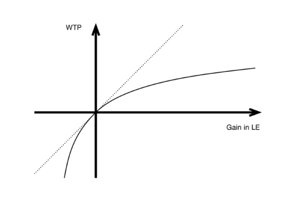
Line graph showing 4 quadrants with an x axis of WTP and y axis of gain in LE. The two lines on the graph both cut through the centre of the quadrant: a diagonal dashed line going up from left to right and a solid curved line.

One caveat to the use of WTP instead of WTA is that there may be circumstances in which WTA is the theoretically appropriate construct (since, for example, a policy is expected to cause or prevent losses in some outcome such as life expectancy). Such an argument is put forward by Jack Knetsch, notably in his 2007 article which argues that “the choice of measure matters” (Knetsch, 2007). Using this line of argument, and if loss aversion is considered an acceptable feature of public preferences, then it is precisely because of the empirical gap between WTA and WTP that the use of the appropriate method becomes imperative. This argument would favour gain-specific and loss-specific values of the VPF and VOLY, and of course such an approach would bring with it substantial issues both practical and ethical.

A second caveat relates to the feasibility of chaining health states using the Standard Gamble. Doing so relies on the assumption that “indirect” and “direct” estimates of the utility of a health state are equivalent. However, some evidence from the health literature have found that indirect estimates of the utility of a health state are higher than direct estimates (Llewellyn-Thomas et al., 1982; Rutten-van Molken et al., 1995; Bleichrodt, 2001; Oliver, 2003). These findings have been used to criticise the descriptive validity of Expected Utility Theory, which is the foundation of the Standard Gamble approach, since they appear to imply that compound lotteries do not reduce to simple equivalents (violations of the Reduction of Compound Lotteries axiom). Caution must therefore be applied in interpreting the results of a chaining study.

A closely-related alternative to the procedure just described would be to estimate the change in life expectancy corresponding to the non-fatal injury/illness by using the QALY-loss associated with the injury/illness, rather than the response to a standard gamble question and, in fact, a variant of this approach was employed by Donald Franklin and reported in Franklin (2015). In particular, using the Carthy et al. (1999) sample mean WTP responses for a quick and complete cure for injuries W (2 or 3 days in hospital; slight to moderate pain; full recovery after 3 or 4 months) and X (2 weeks in hospital; some ongoing pain/discomfort; full recovery after 18 months) updated to 2014 prices, i.e. £3,193 for W and £9,689 for X, and the QALY losses associated with the injuries, i.e. 0.037 for W and 0.2 for X, Franklin estimates the VOLY as £3,193/0.037 = £ 86,297 based on injury W or £9689/0.2 = £48,445 based on injury X.

While Franklin does not attempt to fit an overall V = f(ΔE) valuation function using these results, it seems clear that the difference between the 2 VOLY figures that he derives reflects the high degree of concavity of the underlying function. For the sake of analytical convenience, suppose we assume that the function takes the following simple concave form:

Equation 7

V = a – [b/(c + ΔE)]-

Given that ΔE = 0 => V = 0, it will necessarily be the case that:

Equation 8

a = b/c

so that:

Equation 9

V = bΔE/(c² + cΔE)

In turn, given that ΔE = 0.037 => V = 3193 and ΔE = 0.2 => V = 9689, it follows from equation (9) that b = 3089 and c = 0.1716.

The implied overall V = f(ΔE) valuation function therefore takes the form:

Equation 10

V = 3089ΔE/(0.02945 + 0.1716ΔE)

From this function it is then possible to obtain the implied VOLY = V/ΔE, for any non- marginal increase, ΔE, in remaining life expectancy, as well as the VOLY for genuinely marginal increases, which will be given by the derivative of V with respect to ΔE evaluated at ΔE = 0 (i.e. the marginal rate of substitution of wealth for remaining life- expectancy) and in this case is equal to £104,902. For more substantial non-marginal gains in life-expectancy the implied VOLY decreases significantly, with the figure for a one year gain being only £15,364. It is also possible to infer the implied maximum acceptable decrease in remaining life-expectancy i.e. the reduction in remaining life- expectancy at which V → - ∞ . In this case it is clear that as ΔE → - 0.02945/0.1716 (= - 0.1716), so V → - ∞ , which implies that the maximum acceptable reduction in remaining life-expectancy is just over 2 months.

This estimation of the V = f(ΔE) function is, of course, purely illustrative and has of necessity been based on just 2 different severities of non-fatal injury. The estimation has also used sample mean values for WTP and population mean figures for the avoided QALY losses (and hence the implied gains in remaining life-expectancy), rather than individual responses. Ideally, a full-scale estimation exercise would be based on a larger number of severities of non-fatal injury/illness (for practical purposes, perhaps 3 or 4). In addition, given the potential problems associated with averaging and aggregation inherent in the chained approach - see, for example, Baker et al. (2010) Chapter 6 – it would seem appropriate to estimate the underlying V = f(ΔE) function at both an aggregate and individual level and, when doing so at the aggregate level, to employ sample medians as well as means. In this way it should be possible to identify and allow for the potentially distortional impact of “outlier” responses.

Having set out the main aspects of the theoretical relationship between the VPF and the VOLY and, in addition, considered a number of potential methods that could be harnessed to estimate the latter, we now examine a number of further factors that might inform or affect the relationship between the VPF and VOLY.

4. Other factors that (may) affect the relationship between the VPF and VOLY.

4.1. Perceptions about health at multiple stages of life

It is well-established that people have different perceptions about their future health as they age, particularly if they are considering health over periods which differ greatly in their proximity for example, end of life and current life. This is potentially problematic for the estimation of a VOLY, however derived. However, if younger individuals have a systematic tendency to underestimate their expected health in later years (i.e. to imagine that they will live in a poorer state of health than is actually the case), and hence do not properly reflect their true preferences when considering (and then discounting) these future years, then it may lead to lower VOLYs and (implied) VPFs than might otherwise be the case, and ultimately lead to an underestimate of the appropriate amount of resource that should be allocated to interventions that improve the chance of survival to later years of life. To explore the potential impact of this factor we draw on some evidence from both the broader health preference literature more generally as well as the safety literature that has attempted to investigate this issue.

If later years of life are spent in lower quality of life, as is consistent with at least some empirical evidence (for example, Fritjers and Beatton 2012), then it may be legitimate to down-weight these years compared to earlier years of life to account for this effect, independent of time preference (see Frederick (2006) for a useful discussion of the distinction between the effect of delay on the utility of an outcome when it is received, versus the effect of delay due to time preference).. A meta-analysis by Stock et al. (1983) suggested that age actually uniquely accounts for less than 1% of the variation in reported Subjective Well-Being, suggesting that any down-weighting of future life years for quality may be misguided. In contrast, Frijters and Beatton (2012) used 3 large panel datasets (the British Household Panel Survey, the Household Income Labour Dynamics in Australia, and the German Socio Economic Panel) concluding that in all 3 panels, there is a peak of happiness around age 60 with a sharp decline after age 75. It is indisputable that health status typically declines with age. However, there is no clear reason to suppose that all future life years will be spent in lower quality of life compared to the present.

Even if later years of life really are spent in lower quality of life than earlier years, down- weighting those years will only be acceptable if the degree to which down-weighting happens accurately reflects the actual reduction in quality of life experienced at older ages. However, it is possible that individuals at a younger age might mis-estimate their quality of life when predicting how their life will be at older ages. Specifically, if respondents expect their health, and their quality of life, to be lower in old age than is actually the case, then the value of later life years may be underestimated, resulting in an overall underestimate of the VPF, if based on the stated preferences of the young. Much of the literature regarding how age influences WTP for reductions in fatality risks was outlined in RQIV. However, here we outline the literature specifically relating to the possibility that quality of life at older ages may be underestimated by younger respondents.

An early paper that directly addressed the possibility that there may be a mismatch between predicted and actual quality of life in old age is Johannesson and Johansson (1997). The authors surveyed a random sample of Swedish population and found that expected quality of life at an advanced age is low, relative to the actual average quality of life reported by elderly Swedish people. In the health setting more generally, Sackett and Torrance (1978) provided early evidence to suggest that when non-patients were asked to estimate the impact on their daily lives of becoming a dialysis patient (needing home dialysis for life), the quality of life they predicted was 0.39 (on a 0 to 1 scale representing as bad as death to full health) compared to an actual report of 0.56 from current dialysis patients. Similar results were found by Boyd et al. (1990) for colostomies due to carcinoma of the rectum and Sieff et al. (1999) for HIV.

Clearly then, predictions of the adverse quality of life impacts from health problems tend to be exaggerations of the experienced effects – this links to a related literature exploring affective forecasting errors (see Wilson and Gilbert, 2005 for an overview). In an interesting review, Loewenstein et al. (2003) propose a range of possible explanations for this effect, proposing a model of “projection bias” to account for these phenomena (though their model is applicable well beyond the medical domain).

Loewenstein and Schkade (1999) further suggest that salience may partly explain the discrepancy between anticipated and realised effects on wellbeing – when a young person is asked to value their future years of life, they may focus on the effects of being older than they are now – perhaps including poorer health and lower income – and ignore the ways that their lives may actually stay the same or improve.

In this sub-section, we have addressed the possibility that the WTP for future mortality risk reductions may be erroneously predicted in the context of quality of life, and we have touched upon the broader literature on affective forecasting errors. Overall, it seems that there is limited evidence to suggest that quality of life substantially falls with age until after age 75, when quality of life does appear to fall. It also appears that individuals tend to be overly pessimistic about their quality of life in older age. The way that this may influence the relationship between the VOLY and the VPF will depend on the specific perturbation of the survival function leading to the gain in one year of life expectancy. If the risk reductions are concentrated on later years, then the VOLY may be severely under-estimated if based on the preferences of the young. If, on the other hand, the risk reduction benefits are concentrated in the current period (as is typically associated with the VPF) then there may be less discrepancy between the VOLY and the VPF (both the VOLY and the VPF may still be subject to this excessive deflation, but not to differing degrees).

4.2. Personal time preference rates

A priori, we might expect people at different ages to have different discount rates. This is of profound significance in the case of a VOLY and lea ds to many ethical questions with respect to how to deal with this in the policy arena. One way might be to apply a “time neutral VOLY” in which variations in personal time preferences are offset, thereby generating a VOLY based on a rate which might be considered to reflect a common social time preference. But this is not straightforward in practice. Indeed, there has been little if any research at all into empirical discounting with respect to the VOLY per se. Discounting has been explored empirically to some extent in the context of a VPF and it seems reasonable to assume that some of the insights gleaned in that context carry over to a VOLY.

Indeed, in the theoretical literature the discount rate is a crucial factor in linking the VPF and the VOLY (see, for example, Jones-Lee et al., 2015). The literature on personal time preference rates in the context of fatality risks was extensively reviewed as part of RQIV. To summarise that discussion, a substantial body of evidence suggests that individuals do apply discounting in their evaluation of the benefits of future reductions in their own personal risk of fatality. The rates estimated, which originate mainly from the VPF literature, typically lie in the region of 10% per annum. Despite its theoretical importance, the empirical VOLY literature often sidesteps the elicitation of discounting, either by setting it aside altogether (for example, Desaigues et al., 2007; Vlastachokostas et al., 2011; and Desaigues et al., 2011) or by assuming a discount rate based on theory or policy guidance (e.g. Nielsen, 2010; Chilton et al., 2004; Hammar and Johansson-Stenman, 2004 and Grisolia et al., 2018). The exceptions are Chanel and Luchini (2008) who estimate a discount rate of 6.4% (with different estimates provided depending on the modelling assumptions that are employed) and Chanel and Luchini (2014) who elicit 6.8% in a telephone survey and 18.8% in a face-to-face procedure. Finally, Johannesson and Johansson (1996) elicit a discount rate between 0.3% and 3.4%. Importantly, all of the VOLY estimation assumes a constant, exponential discounting function.

One result common to the empirical discounting studies that elicit personal discount rates at an individual level is the wide variation between subjects in terms of their personal discount rate. Where studied, wide variation also characterises the functional form for discounting that individuals employ (this was the main focus of McDonald et al. (2017) in the context of a VPF for cancer). There exists the possibility that differences in the value of a life year between individuals, when specified in the same way (i.e. resulting from the same perturbation in the survival function) may be in part due to differences in the way that these individuals discount future mortality risk reductions. With appropriate, reliable individual-specific measures of discounting, it may be possible to control for the discounting already present in stated preference estimates of the value of a life year, generating a VOLY that controls for the effects of personal discounting. This value may then be discounted according to a social discount rate deemed appropriate for policymaking, for example the 1.5% rate recommended in UK policymaking for health outcomes. This approach can conceivably be taken to account for non-standard discounting (e.g. hyperbolic discounting), allowing a more normatively desirable exponential function to be imposed on the “time neutral” valuation.

The defensibility of this approach depends on the degree to which individuals’ stated valuations of changes to their own (discounted) life expectancy are considered to be a valid basis for policymaking. Heterogeneity in discount rates (and discount functional forms) might be considered a valid and integral part of public preferences, in which case the “un-discount, re-discount” approach may not be deemed appropriate in defining the social value of a risk reduction for use in policy evaluations. On the other hand, if “excessive discounting” or “non-standard discount functions” are considered to be a bias that distorts individuals’ true underlying values for the changes in risk, then it may be considered appropriate to adjust the values as described. Regarding the appropriateness of “laundering [stated] preferences” to better reflect the underlying, “true” preferences, Harsanyi (1977) stated:

[w]e have to disregard, not only preferences distorted by factual or logical errors, but also preferences based on clearly antisocial attitudes, such as sadism, resentment, or malice

(Harsanyi 1977, 30)

The degree to which high discount rates and/or non-exponential discounting can be counted as “factual or logical errors” is a matter for judgement. For now, we simply state that such an approach is possible.

There also exists a question about how to value changes life expectancy that would not occur until some future time period. The literature relating to this question was also outlined in RQIV. However, in terms of explaining the link between the VPF and the VOLY, discounting of future generations and/or discounting fatality risks that occur in the future is not directly relevant, since the question is about how a VPF can be linked with a VOLY, and not about how the VPF or the VOLY themselves should be discounted for delay. The reader is referred to RQIV for relevant discussions.

4.3. There could be diminishing marginal returns to life years, so the value of 10 extra years is not 10 times the value of 1 extra year – at least in anticipation

Kvamme et al. (2010) examined this issue in the context of cost-effectiveness analysis to address the issue as to whether the health gains used in the denominator of the cost-effectiveness ratio are valued linearly. If so, this would imply constant marginal returns to life years. If not, and instead, marginal utility is increasing for extensions of small duration, then this might affect health care evaluations at different levels due to the mis-specified QALY value formula. An alternative channel would occur if TTO is used, in which case the values could be over or underestimated depending on the durations specified in the questions. Overall, there is a danger that single programmes delivering small QALY gains may be judged as cost-ineffective, whilst programmes offering ‘bundles’ of such small gains may generate a different result^{[footnote 5]}.

In contrast with previous studies, Kvamme et al. (2010) examined relative preferences (of a representative sample of the Norwegian population aged 40 to 59 years) over small gains i.e. 1 week to 1 year, added to a hypothesised limited remaining life expectancy of 1 year or 10 years. These gains were presented as certain, as opposed, to risky amounts to control for the cognitive problems associated with processing small probabilities. Results from close-ended WTP questions showed that respondents were more likely to accept interventions offering a larger (rather than a smaller) life extension. Data from a follow-up open ended WTP question exhibited either constant or increasing utility over health gains. However, the authors point to some difficulties in interpretation: responses suggesting constant WTP across larger life-gains may be affected by biting budget constraints, so this pattern may mask increasing marginal utility over life-gains. Further, decreasing WTP does not necessarily reflect decreasing marginal utility over lifetime. It is also impossible to determine how potential diminishing marginal utility of income (rather than an assumed constant marginal utility of income) affects responses. However, assuming some degree of overall income effects, the authors conservatively concluded that at least 65% of respondents exhibit increasing marginal utility over health gains.

Based on this evidence, it is not possible to be definitive on whether marginal returns to increases in life expectancy are constant or increasing. This is partly due to the lack of risk in the above framework, the fact that a relative valuation framework was used^{[footnote 6]} and potential confounds relating to the impact of potential diminishing marginal utility of income.

It should also be noted that the results of the study reported in Franklin (2015), which employed the WTP responses from the stated-preference survey reported in Carthy et al. (1999) – together with the analysis set out above in Section 4.2 – clearly indicate that individual WTP is an increasing but strictly concave function of the gain in life expectancy, which implies diminishing returns to gains in life expectancy, though this is almost certainly a reflection of biting budget constraints.

4.4. The utility opportunity cost of money may vary with age

The potential issue here is that older people may have fewer concerns for saving their money for as long as a younger person would, and hence may be willing to spend more on extending life expectancy, ceteris paribus.

Underlying a conventional Cost Benefit Analyses (CBA) is an important assumption: that marginal social welfare of income is constant across individuals (i.e. $1 buys the same amount of utility for a rich and a poor individual) (Baker et al., 2009). An implication of this assumption is that marginal social welfare of income (hereafter named marginal utility of income) is constant across age groups and health states. In Baker et al., (2009), the assumption of constant marginal utility of income is relaxed and the authors demonstrate that the application of a ‘common VSL’ can be theoretically justified by assuming a constant marginal welfare of survival probability.

However, in the wider literature it has been suggested that health status impacts on the marginal utility of income (consumption) and we therefore have health state dependent utility functions. According to Gyrd-Hansen (2017), the marginal utility of consumption may increase with poorer health (positive state dependence), because of increased reliance on costly entertainment and luxury in own home, or alternatively, poorer health may entail lower marginal utility of consumption (negative state dependence) because of the constraints that poor health may have on activities such as travel and sport. This study found that improved health increases the marginal utility of income for intermediate health states whereas this is not the case for less and more severe health states and identified 8 additional studies which have also examined this issue (Edwards, 2008; Lillard and Weiss, 1997; Sloan et al., 1998; Viscusi and Evans, 1990; Evans and Viscusi, 1991; Finkelstein et al., 2009, 2013; Levy and Nir, 2012; Tengstam, 2014). These studies demonstrate contradictory evidence as 3 of these studies found negative state dependence, 4 studies show positive state dependence and one study shows no state dependence.

Turning to the literature studying preferences for end-of-life treatment (see Pennington et al., 2015), it has been argued that for a person with a fatal illness money is, subject to bequest motives, more or less worthless. The implication is that it would be natural (and utility maximising) for that person to express a high willingness-to-pay for a small chance of a cure. This is also referred to as the ‘Dead Anyway Effect’ (Pratt & Zeckhauser 1996). Another way of describing this is that if the opportunity cost of spending is zero when there is no value of leaving resources behind when dead, an individual is willing to spend all of his wealth to prolong life, though perhaps just briefly (Becker et al., 2007). However, as explained in Pennington et al. (2015), it is worth mentioning that if a health and safety intervention is financed by a common pool of funds (public or private), it is the general public (who are not facing death in the near future) who are to finance the intervention, and for whom the opportunity cost of spending additional dollars on terminal illness programmes may well be high in terms of other programmes forgone.

In summary, there does not seem to be compelling evidence at this present time to relax the assumption that marginal social welfare of income is constant across individuals when estimating a VOLY – given that the average respondent is not at the end of life.

4.5. Individuals of different ages might value an additional year of life differently or other reasons than those above

The broader health economics literature has explored this issue primarily from a “societal” or “citizen” perspective^{[footnote 7]} using Discrete Choice or Person Trade-Off frameworks rather than an individual-based, WTP-based perspective. Whilst this perspective is not incorrect per se as a method for preference elicitation, the resulting measures are problematic if used in CBA since their compliance with the underlying tenets of that framework cannot be clearly established. Nevertheless, these studies do provide some insights into equity weighting^{[footnote 8]} that help in explaining how values might change over time. Reviews of the literature indicate that, in general there appears to be a preference for providing health and/or safety benefits to the young over benefits to the elderly (Gu et al., 2015; Whitty et al., 2014) although a number of studies find instead that preferences for age follow an inverted U pattern implying that those of a working age are preferred more than the elderly and the young (Baker et al., 2010; Charny et al., 1989; Cropper et al., 1994; Diederich et al., 2012; Jelsma et al., 2002; Palanca-Tan, 2013; Petrou et al., 2013; Whitty et al., 2014b). The reason(s) for this are unspecified but could relate to: working age adults having dependents (Murray and Lopez, 1994) and the elderly being deemed as having had their ‘fair innings’ (Williams, 1997).

5.6. There might be some fixed level of disutility associated with death which is reflected in the VPF but not necessarily the VOLY

This possibility might arise since, as noted by the Contractor, the VPF tends to be used in contexts where there is a risk of sudden and untimely death, whereas VOLYs tend to be associated with changes in life expectancy. Thus, in other words, individuals themselves may naturally think in terms of VPFs in some circumstances and VOLYs in others, even if the former were applied to estimate the value of a life year resulting from a reduction in the risk of death in the forthcoming period.

It is unfortunately the case that the literature tells us nothing about people’s relative aversion to each type of risk. It is well-documented that people fear different risks of premature death with different degrees of fear or ‘dread’ (see, for example, Slovic et al., 1981; Thomas, 1981; Mendeloff and Kaplan, 1990; McDaniels et al., 1992), Savage, 1993; Tolley et al., 1995 and Jones-Lee and Loomes, 1995). Whether any of these findings extend to arguably less emotive risks or risks without media amplifying characteristics is an open question and one that cannot be answered definitively given currently available evidence.

5. Summary

In the chapter, we have provided a formal definition of the VOLY and set out its relationship to the VPF in the case where the former is derived indirectly from the latter (by dividing it by remaining life expectancy). In doing so, we have clarified that the only way in which remaining life expectancy can be increased is by reducing the hazard rate in the forthcoming period and/or future periods. Further, we have shown that the assumption that a VPF is the sum of an individual’s (discounted) VOLYs is inappropriate, although at the aggregate level it is not incorrect to divide a VPF by (remaining) life expectancy to derive a VOLY.

In relation to how the WTP-based value per statistical year’s gain in undiscounted remaining life-expectancy generated by ongoing hazard rate reductions can be expected to relate to the value derived for a year’s gain in undiscounted remaining life- expectancy generated by a reduction in the coming year’s hazard rate, we established – under reasonable assumptions about personal discounting – that since a gain in undiscounted life-expectancy generated by a delayed hazard rate reduction will yield a smaller gain in discounted expected utility than the same gain in undiscounted life- expectancy generated by an earlier hazard rate reduction, then a lower VOLY would apply to the former undiscounted life expectancy gain (of the same duration).

The method for deriving a VOLY described above is based on the assumption that the hazard rate only changes in the coming year and, further, that the marginal hazard rate reductions are equal across all affected individuals. If the latter assumption is relaxed, but the new risk reductions set to ensure that all affected individuals enjoy the same marginal life expectancy gain, then the appropriate measure for the aggregate WTP for an aggregate gain of one year of life expectancy (i.e. the VOLY) is the mean of the ratio, m_i /E_i^{[footnote 9]}, rather than, as in the previous case, the mean of m_i divided by the mean of E_i. The magnitude of the mean of this ratio relative to the magnitude of the ratio of the means of m_i and E_i (the measure under the original assumptions) will depend on the covariance between the m_i and E_i. As pointed out, the 2 VOLYs will be approximately equal only if m_i and E_i are positively correlated. Empirical evidence does suggest that a positive correlation exists from middle age onwards so on these grounds it seems reasonable to assume that the 2 measures should not differ greatly. This argument holds for both undiscounted and discounted life expectancy.

Further, Jones-Lee et al. (2015) showed that if remaining life-expectancy is itself also computed on a discounted basis using the same discount rate as that applied to anticipated future utilities, then the VOLY will be completely independent of the distribution of future hazard rate reductions that generate the gain in discounted life- expectancy and will also be independent of the age.

We then established that a number of potential techniques exist, at least some of which have the potential to be taken forward to new primary research to value a VOLY. Direct elicitation methods are based on asking people to value life expectancy gains and/or associated reductions in the hazard rate. Indirect methods – which are designed to avoid the problems inherent in valuing small risks – are based around ‘chaining’. In these approaches, the evaluation task is broken down into 2 components in which the respondent first values the opportunity to recover quickly from an injury or minor health problem. This response is then ‘chained’ to (for example) a standard gamble (in which they indicate the risk of death (q) they are willing to take in order to enjoy the corresponding chance (1-q) of a complete cure or avoided QALY-losses, either of which can be interpreted as the value of the proposed life expectancy gain. Problems that might arise (or have arisen) were noted.

Finally, we established that, in most cases, the literature pertaining to the factors included in 5.1-5.6 was too sparse or inconclusive to generate definitive findings. Even in the case of time preferences (and age) much is yet to be learned.

References

Baker, R., Bateman, I., Donaldson, C., Jones-Lee, M., Lancsar, E., Loomes, G., Mason, H., Odejar, M., Pinto Prades, J.L., Robinson, A., Ryan, M., Shackley, P., Smith, R., Sugden, R. and Wildman, J. (2010).Weighting and valuing quality-adjusted life-years using stated preference methods: preliminary results from the social value of a QALY project. Health Technology Assessment, 14, 1-162.

Baker R, Chilton S.M., Jones-Lee M.W. and Metcalf H.R.T. (2009). Valuing lives equally: defensible premise or unwarranted compromise? Journal of Risk and Uncertainty, 36, 125-138.

Baker R, Chilton S.M., Jones-Lee M.W. and Metcalf H.R.T. (2009). Valuing lives equally in a benefit-cost analysis of safety projects: a method to reconcile theory and practice. Safety Science, 47, 813-816.

Becker, G., Murphy, K., and Philipson, T. (2007). The value of life near its end and terminal care. National Bureau of Economic Research.

Bleichrodt, H. (2001). Probability weighting in choice under risk: an empirical test. Journal of Risk and Uncertainty, 23(2), 185-198.

Bleichrodt, H., and Pinto Prades, J. L. (2009). New evidence of preference reversals in health utility measurement. Health Economics, 18(6), 713-726.

Boyd, N. F., Sutherland, H. J., Heasman, K. Z., Tritchler, D. L., and Cummings, B. J. (1990). Whose utilities for decision analysis? Medical Decision Making, 10(1), 58-67.

Carthy, T., Chilton, S., Covey, J., Hopkins, L., Jones-Lee, M., Loomes, G., Pidgeon, N. and Spencer, A. (1999). On the contingent valuation of safety and the safety of contingent valuation: Part 2 – the CV/SG “chained” approach. Journal of Risk and Uncertainty, 17 (3), 187-213.

Chanel, O. and Luchini, S. (2008). Monetary values for air pollution risk of death: A contingent valuation survey. HAL open access report.

Chanel, O. and Luchini, S. (2014). Monetary values for risk of death from air pollution exposure: a context-dependent scenario with a control for intra-familial altruism. Journal of Environmental Economics and Policy, 3(1), 67-91.

Chapman, G. B., and Johnson, E. J. (1995). Preference reversals in monetary and life expectancy evaluations. Organizational Behavior and Human Decision Processes, 62(3), 300-317.

Charny, M.C., Lewis, P.A. and Farrow, S.C. (1989). Choosing who shall not be treated in the NHS. Social Science and Medicine, 28, 1331-1338.

Chilton, S., Covey, J., Jones-Lee, M., Loomes, G., and Metcalf, H. (2004). Valuation of health benefits associated with reductions in air pollution. Final Report. DEFRA, London.

Cropper, M.L., Aydede, S.K. and Portney, P.R. (1994). Preferences for life saving programs: how the public discounts time and age. Journal of Risk and Uncertainty, 8, 243-265.

Desaigues, B., Rabl, A., Ami, D., My, K.B., Masson, S., Salomon, M.A. and Santoni, L. (2007). Monetary value of a life expectancy gain due to reduced air pollution: Lessons from a contingent valuation in France. Revue d’économie Politique, 117(5), 675-698.

Desaigues, B., Ami, D., Bartczak, A., Braun-Kohlová, M., Chilton, S., Czajkowski, M., Farreras, V., Hunt, A., Hutchison, M., Jeanrenaud, C. and Kaderjak, P. (2011). Economic valuation of air pollution mortality: A 9-country contingent valuation survey of value of a life year (VOLY). Ecological indicators, 11(3), 902-910.

Diederich, A., Swait, J. and Wirsik, N. (2012). Citizen participation in patient prioritization policy decisions: an empirical and experimental study on patients’ characteristics. Plos One 7(5): e36824. doi:10.1371/journal.pone.0036824.

Dolan, P., and Kind, P. (1996). Inconsistency and health state valuations. Social Science and Medicine, 42(4), 609-615.

Dolan. P., Shaw, R., Tsuchiya, A., and Williams, A. (2005). QALY maximisation and people’s preferences: a methodological review of the literature. Health Economics 14(2), 197-208.

Dow, W.H., Philipson, T. and Sala-i-Martin, X. (1999). Longevity complementarities under competing risks. The American Economic Review, 89 (5), 1358-137.

Edwards R.D. (2008). Health risk and portfolio choice. Journal of Business and Economic Statistics, 26(4), 472–485. Evans W.N. and Viscusi W.K. (1991). Estimation of state-dependent utility functions using survey data. Review of Economics and Statistics, 73(1), 94–104.

Franklin, D. (2015). Derivation of the monetary value of a QALY or SLY. Unpublished Manuscript.

Finkelstein A., Luttmer E.F.P. and Notowidigdo M.J. (2009). Approaches to estimating the health state dependence of the utility function. American Economic Review: Papers and Proceedings, 99(2), 116–121.

Finkelstein A., Luttmer E.F.P. and Notowidigdo M.J. (2013). What good is wealth without health? The effect of health on the marginal utility of consumption. Journal of the European Economic Association, 11, 221–258.

Frijters, P., and Beatton, T. (2012). The mystery of the U-shaped relationship between happiness and age. Journal of Economic Behavior & Organization, 82(2-3), 525-542.

Grether, D.M and Plott, C. R. (1979). Economic theory of choice and the preference reversal phenomenon. The American Economic Review, 69(4), 623-638.

Grisolía, J.M., Longo, A., Hutchinson, G. and Kee, F. (2018). Comparing mortality risk reduction, life expectancy gains, and probability of achieving full life span, as alternatives for presenting CVD mortality risk reduction: A discrete choice study of framing risk and health behaviour change. Social Science and Medicine. 211, 164- 174.

Gu, Y., Lancsar, E., Ghijben, P., Butler, J.R. and Donaldson, C. (2015). Attributes and weights in health care priority setting: a systematic review of what counts and to what extent. Social Science and Medicine, 146(4), 1-52.

Gyrd-Hansen, D. (2017). A stated preference approach to assess whether health status impacts on marginal utility of consumption. Health Economics, 26, 1224-1233.

Gyrd-Hansen, D. and Kristiansen, I.S. (2007). Preferences for ‘life-saving’ programmes: small for all or gambling for the prize? Health Economics, 14(2), 197- 208.

Hammar, H. and Johansson‐Stenman, O. (2004). The value of risk‐free cigarettes–do smokers underestimate the risk? Health Economics, 13(1), 59-71.

Hammitt, J. and Tunҫel, T. (2015). Preferences for life-expectancy gains: Sooner or later? Journal of Risk and Uncertainty, 51 (1), 79-101.

Harsanyi, J. C. (1977). Rule utilitarianism and decision theory. Erkenntnis, 11(1), 25- 53.

Horowitz, J.K. and McConnell, K.E. (2002). A review of WTA/WTP studies. Review of Environmental Economics and Management, 44 (3), 426 - 447.

Jelsma, J., Shumba, D., Kristian, H., De Weerdt, W. and De Cock, P. (2002). Preferences of urban Zimbabweans for health and life lived at different ages. Bulletin - World Health Organisation, 80, 204-209.

Johannesson, M. and Johansson, P.O. (1996). To be, or not to be, that is the question: an empirical study of the WTP for an increased life expectancy at an advanced age. Journal of Risk and Uncertainty, 13(2), 163-174.

Johannesson, M. and Johansson, P. O. (1997). Quality of life and the WTP for an increased life expectancy at an advanced age. Journal of Public Economics, 65(2), 219-228.

Jones-Lee, M.W., Hammerton, M. and Philips, P.R. (1985). The value of safety: Results of a national sample survey. The Economic Journal, 95, 49-72.

Jones-Lee, M. and Loomes, G. (1995). Scale and context effects in the valuation of transport safety. Journal of Risk and Uncertainty, 11(3), 183-203.

Jones-Lee, M., Loomes, G. and Spackman, M. (2007) Human costs of a nuclear accident: Final report Health and Safety Executive. London, NERA Economic Consulting.

Jones-Lee, M., Chilton, S., Metcalf, H. and Nielsen, J. S. (2015). Valuing gains in life expectancy: Clarifying some ambiguities. Journal of Risk and Uncertainty, 51 (1), 1-21.

Kahneman, D., and Tversky, A. (1979). Prospect Theory: An Analysis of Decision under Risk. Econometrica, 47(2), 263-292.

Knetsch, Jack L. (2007). Biased valuations, damage assessments, and policy choices: The choice of measure matters. Research in Law and Economics. Emerald Group Publishing Limited, 345-358.

Kvamme, M.K., Gyrd-Hansen, D., Abel Olsen, J., and Kristiansen, I.S. (2010). Increasing marginal utility of small increases in life-expectancy? Results from a population survey. Journal of Health Economics, 29, 541-548. Levy M, Nir A.R. (2012). The utility of health and wealth. Journal of Health Economics 31, 379–392.

Lichtenstein, S. and Slovic, P. (1971). Reversals of preference between bids and choices in gambling decisions. Journal of Experimental Psychology, 89(1), 46-55.

Lillard L.A. and Weiss Y. (1997). Uncertain health and survival: effects on end-of-life consumption. Journal of Business and Economic Statistics, 15(2), 254–268.

Llewellyn-Thomas, H., Sutherland, H. J., Tibshirani, R., Ciampi, A., Till, J. E., and Boyd, N. F. (1982). The measurement of patients’ values in medicine. Medical Decision Making, 2(4), 449-462.

Lloyd, A. J. (2003). Threats to the estimation of benefit: are preference elicitation methods accurate? Health Economics, 12(5), 393-402.

Loewenstein, G. and O’Donoghue, T., and Rabin, M. (2003). Projection bias in predicting future utility. The Quarterly Journal of Economics, 118(4), 1209-1248.

Loewenstein, G., and Schkade, D. (1999). Wouldn’t it be nice? Predicting future feelings. Well-being. The Foundations of Hedonic Psychology, 85-105.

Mason, H., Jones-Lee, M. & Donaldson, C. (2009). Modelling the monetary value of a QALY: A new approach based on UK data. Health Economics, 18, 933 – 950.

McDaniels, T.L., Kamlet, M.S. and Fischer, G.W. (1992). Risk perception and the value of safety. Risk Analysis, 12, 495-503.

McDonald, R.L., Chilton, S.M., Jones-Lee, M.W. and Metcalf, H.R.T. (2017). Evidence of variable discount rates and non-standard discounting in mortality risk valuation. Journal of Environmental Economics and Management, 82, 152-167.

Mendeloff, J. and Kaplan, R.M. (1990). Are twenty-fold differences in ‘lifesaving’ costs justified? A psychometric study of the relative value placed on preventing deaths from programs addressing different hazards” In Cox L.A. Jr. and Ricci, D.F. (eds), New Risks, Plenum Press, New York.

Murray, C.J.L. and Lopez, A.D. (eds.) (1994). Global Comparative Assessments in the Health Sector: Disease Burden, Expenditures and Intervention Packages. WHO.

Nielsen, J.S. (2010). Approaching the value of a life year: empirical evidence from a Danish contingent valuation survey. Nationaløkonomisk Tidsskrift, 148(1), 67-85.

Nielsen, J. S., Chilton, S., Jones-Lee, M. and Metcalf, H. (2010) How would you like your gain in life expectancy to be provided? An experimental approach. Journal of Risk and Uncertainty, 41 (3), 195-218.

Nielsen, J. S., Chilton, S., Gyrd-Hansen, D., Jones-Lee, M. Liu, J. and Metcalf, H. (2016). Eliciting individual preferences for end-of-life treatments. Paper presented at the Society of Benefit Cost Analysis Annual Conference, Washington, DC (March).

Oliver, A. (2003). The internal consistency of the standard gamble: tests after adjusting for prospect theory. Journal of Health Economics, 22(4), 659-674.

Olsen J.A. (2000). A note on eliciting distributive preferences for health. Journal of Health Economics, 19(4), 541-550.

Palanca-Tan, R. (2013). Age preferences for life-saving programs: using choice modelling to measure the relative values of statistical life. Singapore Economic Review, 58 (2) 1350008 (15 pages).

Pennington, M., Baker, R., Brouwer, W., Mason, H., Hansen, D. G., Robinson, A. and Donaldson, C., (2015). Comparing WTP values of different types of QALY gain elicited from the general public. Health Economics, 24(3), 280-293.

Petrou, S., Kandala, N.B., Robinson, A. and Baker, R. (2013). A person trade-off study to estimate age-related weights for health gains in economic evaluation. Pharmacoeconomics, 31, 893-907.

Pratt, J.W. and Zeckhauser, R.J., (1996). Willingness to pay and the distribution of risk and wealth. Journal of Political Economy, 104(4), 747-763.

Rodriguez-Miguez, E. and Pinto-Prades, J.L. (2002). Measuring the social importance of concentration or dispersion of individual health benefits. Health Economics, 11(1), 43-53.

Rutten-van Mölken, M. P., Bakker, C.H., van Doorslaer, E. K., and Van Der Linden, S. (1995). Methodological issues of patient utility measurement: Experience from 2 clinical trials. Medical Care, 33(9), 922-37.

Sackett, D. L., and Torrance, G. W. (1978). The utility of different health states as perceived by the general public. Journal of Chronic Diseases, 31(11), 697-704.

Savage, I. (1993). An empirical investigation into the effect of psychological perceptions on the willingness-to-pay to reduce risk. Journal of Risk and Uncertainty, 6, 75-90.

Sieff, E. M., Dawes, R. M., and Loewenstein, G. (1999). Anticipated versus actual reaction to HIV test results. The American journal of Psychology, 112(2), 297.

Sloan F.A., Viscusi W.K., Chesson H.W., Conover C.J., and Whetten-Goldstein K. (1998). Alternative approaches to valuing intangible health losses: the evidence for multiple sclerosis. Journal of Health Economics, 17(4), 475–497.

Slovic, P.B., Fischoff, B. and Lichtenstein, S. (1981). Perceived risk: psychological factors and social implications” in Warner, F. (ed) The Assessment and Perception of Risk, Proceedings of the Royal Society, 376, 17-34, London: The Royal Society.

Stock, W. A., Okun, M. A., Haring, M. J., and Witter, R. A. (1983). Age differences in subjective well-being: A metaanalysis. In Light, R. J. (Ed.), Evaluation Studies: Review Annual, 8, 279–302, Beverly: Sage.

Sumner, W., and Nease Jr, R. F. (2001). Choice-matching preference reversals in health outcome assessments. Medical Decision Making, 21(3), 208-218.

Tengstam S. (2014). Disability and marginal utility of income: evidence from hypothetical choices. Health Economics, 23, 268–282.

Thomas, K. (1981). Comparative risk perceptions: how the public perceives the risk and benefits of energy systems” in Warner, F. (ed) The Assessment and Perception of Risk, Proceedings of the Royal Society, 376, 35-50 London: The Royal Society.

Tolley, G., Kenkel, D and Fabian, R. (1995) Valuing Health for Policy. University of Chicago Press, Chicago. Tversky, A., and Kahneman, D. (1992). Advances in prospect theory: Cumulative representation of uncertainty. Journal of Risk and Uncertainty, 5(4), 297-323.

Vlachokostas, C., Achillas, C., Slini, T., Moussiopoulos, N., Banias, G. and Dimitrakis, I. (2011). Willingness to pay for reducing the risk of premature mortality attributed to air pollution: a contingent valuation study for Greece. Atmospheric Pollution Research, 2(3), 275-282.

Viscusi W.K. and Evans W.N. (1990). Utility functions that depend on health status: estimates and economic implications. American Economic Review, 80(3), 353–374.

Whitty, J.A., Lancsar, E., Rixon, K., Golenko, X. and Ratcliffe, J. (2014). A systematic review of stated preference studies reporting public preferences for healthcare priority setting. The Patient-Patient-Centered Outcomes Research, 7 (4), 365-386.

Whitty, J.A., Ratcliffe, J., Chen, G. and Scuffham, P.A. (2014b). Australian public preferences for the funding of new health technologies: a comparison of discrete choice and profile case best-worst scaling methods. Medical Decision Making, 34, 638-654.

Williams, A. (1997). Intergenerational equity: an exploration of the `fair innings’ argument. Health Economics, 6, 117-132.

Wilson, T. D., and Gilbert, D. T. (2005). Affective forecasting: Knowing what to want. Current Directions in Psychological Science, 14(3), 131-134.

1. At odds with current practice as recommended in HMT Green Book. ↩

2. Empirical values from this framework are reviewed in RQI. ↩

3. Each year’s survival probability is multiplied by 1, representing 1 year. ↩

4. As the CBA framework sum values across the relevant population we follow this convention and present the basic presentation of the VOLY on the aggregate level which is also in line with the UK definition of VPF, see the discussion in Jones-Lee et al., (1985). Following the presentation in Jones-Lee et al., (1985), let mmii = MRS of wealth for probability of death, δδppii = individual risk reduction and VPF = Σii mmii δδppii . If δδppii = 1/n, then VPF = (1/n)Σii mmii. Hence under these conditions, the VPF is the mean MRS of wealth for probability of death and it is therefore needed to establish the MRS at the individual level. ↩

5. A VOLY analogue might be that a life expectancy gain generated by a single period risk reduction (occurring now or in the future) might be valued at zero by respondents, and yet a life-expectancy gain generated by more than one such single-period risk reduction may be given a positive value. ↩

6. This was entirely appropriate for their investigation; the issue here is simply that results may have be different (or not) had absolute values been elicited for the different durations of life-gain. ↩

7. Whilst not incorrect per se as a method for preference elicitation, the resulting measure are problematic if used in benefit-cost analysis since their compliance with the underlying tenets of that framework cannot be clearly established. ↩

8. See RQIII for a more detailed consideration of equity weights. ↩

9. Where, as previously defined, m_i is the mean marginal rate of substitution of the i^th individual’s wealth for his/her risk of death during the coming year and E_i is remaining life expectancy. ↩