The long shadow of deprivation - technical annex (HTML)

Question 1

Introduction

Accepted Answer

The key principle behind social mobility is that everyone gets a fair chance of success in life, whether in big cities or small towns, and whether your parents are rich or poor. Most existing research focuses on the national story: how factors such as parents’ income and class affect their children’s lives, nationwide. Very little research has been done to understand how the picture varies in different places and why.^{[footnote 1]} This report sheds light on this important issue for the first time, highlighting large differences in opportunities around the country.

Promoting social mobility has been an important policy objective of all governments over the past decade, from Nick Clegg’s claim that ‘Improving social mobility is the principal goal of the Coalition government’s social policy’ to the current government’s ‘levelling up’ agenda.

Successive administrations have targeted a fairer and more equal society, in which circumstances of birth – including the family you are born into and the place where you grew up – do not matter.

But does someone raised in Manchester have the same opportunities as a similar individual raised in Malvern Hills? While regional disparities in social mobility and opportunities have been recognised in policy at an increasing rate over the past decade – from David Cameron and George Osborne’s Northern Powerhouse, to Theresa May’s Opportunity Areas, Industrial Strategy and Midlands Engine – there has been little evidence on how the impact of childhood family circumstances on later life earnings differs at the local level. The first objective of this report is to describe the importance that place plays in determining outcomes. The second objective is to consider why opportunities vary across place, examining the role of two important factors for social mobility: education and the labour market.

We find that geography matters for social mobility. Where you are born makes a difference to how much money you make and to the education you achieve. There are significant differences in how disadvantaged sons^{[footnote 2]} who grew up in different local authorities (LAs) fare in the labour market, as well as significant differences in the size of the pay gap between sons from the most and least disadvantaged families. There are also differences in the educational achievement of sons from the most and least deprived backgrounds across local authorities, with areas with the lowest pay gaps also tending to have the lowest gaps in educational achievement.

Some of the differences between areas defy easy explanation. This is not a simple story of north versus south, or urban versus rural. Local authorities with the worst outcomes include cities like Sheffield and Bradford. And the perception of London outperforming other regions is only partly borne out, since the capital has boroughs with sharp contrasts in the outcomes of rich and poor children.

Across the country, the gaps in educational achievement between sons from the most and least deprived families explain the vast majority of the later gap in earnings between those groups.

However, the education gaps explain a broadly stable amount of pay gaps across local authorities – and so a much smaller total proportion of the pay gap in areas where pay gaps are large (less mobile areas) compared with areas where pay gaps are small (more mobile areas). In fact, in the most mobile areas education gaps can explain virtually all of the pay gaps. But in less mobile areas, there are other factors at play that drive differences in earnings between sons from poor and rich families, even when they have the same education. This key finding suggests that in order to ‘level up’ between places, we need to look beyond the education system to understand why equally achieving sons have different opportunities in the labour market.

While our analysis cannot pinpoint any specific factors, these could include the role of family connections and finances in finding good jobs, the role of schools and colleges in adequately preparing pupils for the local labour market, and the role of employers in adopting inclusive recruitment policies. They could also include regional differences in internal migration flows and the possibility that deprived sons growing up in less equal areas are less likely to move to areas with better prospects than sons growing up in more equal areas. Further investigation of the precise nature of these factors is needed in order to understand how to equalise social mobility across the country.

This analysis is made possible by the recent linkage of administrative education data (National Pupil Database and Higher Education Statistics Authority) and earnings and benefits records (HM Revenue and Customs and the Department for Work and Pensions) in the Longitudinal Education Outcomes (LEO) dataset. These data, which have never previously been used to study how opportunities are passed across generations, allow us to link all state-educated sons born between 1986 and 1988 who attended school in England to the area where they grew up and track their educational and labour market experiences. This allows us to measure the gap in adult earnings between sons from the most and least deprived families who grew up in the same area, and compare the earnings of sons from disadvantaged families across areas. We measure the link between family circumstances at age 16 and later labour market earnings at age 28 for over 800,000 sons, across the 326 lower-tier local authorities in England.

Policy context of our cohort

Our group of ‘Millennials’ were born between 1986 and 1988 during a period in which income inequality had just increased considerably. Home ownership also increased during this period through the Right to Buy scheme, which meant that social housing tenants could buy their home for the first time. By 1987, more than one million council-owned homes had been purchased by their tenants.

The 1988 Education Reform Act, which introduced considerable changes to the education system, set the stage for the cohort’s entire education experience. Increased accountability and transparency were key components of the reform, which saw the introduction of league tables and parental choice as ways to bring market forces into the education system by encouraging schools to compete for pupils. Our cohort entered primary school as the New Accountability Framework was introduced in 1992, which established Ofsted to ensure compliance in schools. For their parents, the 1991 recession saw high rates of unemployment and inflation. The crash, alongside the failed Exchange Rate Mechanism (ERM) experiment of 1992, led to high interest rates and falling house prices, which caused considerable negative equity problems for many mortgage holders.

The secondary school journey of our cohort coincided with a period which saw large increases in investment in education. Some of the initiatives which were introduced then, such as Excellence in Cities (1999), coincided with the secondary school experiences of our cohort. Other initiatives such as Teach First (2002) and the London Challenge (2003) were introduced when this group were in their final years of compulsory education (2002 to 2004).

Our Millennial sons entered post-compulsory schooling at a time of increased costs of higher education, with the increase in university fees from £1,000 to £3,000 in 2006. But they also experienced increased support, through the Education Maintenance Allowance (EMA, 2001 to 2004) and the introduction of income-contingent loans for fees in higher education, meaning that fees no longer had to be paid up-front. Grants were reintroduced to cover living costs in 2005, while maintenance loans increased in generosity in 2006.
The ‘Great Recession’ of 2008 hit at a time when our cohort were either establishing themselves in (for school leavers) or just entering (for those who went on to higher education) the labour market. The period of austerity that followed the Great Recession meant a contraction of public services. While in the years following the recession unemployment slowly recovered to pre- recession levels, there was a marked rise in zero-hours contracts and a shift to the gig economy for the lowest paid.

This period also saw the Social Mobility Commission come into existence. The then-named Child Poverty Commission was created following the 2010 Child Poverty Act as an independent body to monitor and provide advice on the then-government’s Child Poverty Strategy. To ensure that the issue of child poverty was considered within the broader context of children’s life chances, the Commission’s remit was extended in 2011 to include social mobility, before it was renamed the Social Mobility Commission in 2016.

At the time that we measure the adult earnings of our cohort of sons at age 28 (2014 to 2016), the economy was recovering and new schemes were planned to boost regional economies and education systems, including the Northern Powerhouse, Industrial Strategy, and investment in Opportunity Areas. Much like some of the education investments introduced in the 2000s, these policy interventions are likely to have been introduced too late for their impact to form part of this analysis. More recent events such as Brexit and COVID-19 fall out of the scope of what is measured here.

Roadmap for the technical report

We start this technical report with a discussion of the related academic literature to set the report in context. In Sections 2 and 3, we describe our data and methodology in detail. Section 4 presents our estimates of intergenerational mobility at the national level to ground our report in the related literature and provide a baseline for comparison with our area-level estimates. Section 5 presents the regional differences in the earnings of disadvantaged sons, and relative mobility rates (pay gaps between the most and least deprived sons) across England. Next, the report turns to investigating the reasons why mobility varies across areas. Section 6 discusses why education is likely to matter in the transmission of earnings from parents to sons and presents our estimates of the role that education plays in driving intergenerational transmission at the national level. Section 7 investigates the role that education plays in explaining the regional differences in mobility we observe across England. Section 8 concludes with a discussion of future policy challenges. We discuss what this research can tell us in terms of what and who policy-makers should focus on and how our findings tie in with the current policy landscape, including recent initiatives such as the Towns Fund and Opportunity Areas. We outline priorities for future research and describe the data needed to make it possible.

Figure 1.1: Policy timeline

Question 2

1.  Related research

Accepted Answer

A large multi-disciplinary literature documents and analyses the sources of intergenerational persistence in economic and social outcomes. For a long time, much of this literature has focused on estimating measures of intergenerational mobility at the national level in different countries. The broad consensus from this literature is that, in international terms, the UK has fairly low mobility. For example, among OECD countries, the UK has one of the lowest intergenerational income elasticities – a commonly used measure of the relationship between parent and child’s income – rivalled only by the US (Dearden, Machin and Reed, 1997; Solon, 2002; Jantti et al., 2006; Corak, 2006; Jerrim and Macmillan, 2015). Moreover, there seems to have been little improvement in intergenerational mobility in the UK over time. In fact, recent research shows that intergenerational income mobility has fallen between cohorts born in the 1950s and cohorts born in the 1990s (Blanden et al., 2004; Gregg, Macmillan and Vittori, 2017; Bell et al., 2018). For example, Blanden et al. (2004) document a 50% decline in intergenerational income mobility between the 1958 and 1970 cohorts.

High intergenerational persistence is not only apparent in terms of income; gaps between children born in deprived families and their more affluent counterparts are evident in an array of outcomes, including educational attainment, socio-emotional skills and health (Macmillan et al, 2018; Zylberstztejn et al., 2018). These socio-economic gaps open up early (Chowdry et al., 2013; Waldfogel, 2013) and have been shown to explain a significant fraction of gaps in later outcomes, such as university participation (Crawford et al., 2016) and income (Blanden, Gregg and Macmillan, 2007).

A crucial question in this literature relates to the drivers of intergenerational persistence. A vast number of hypotheses have been proposed to explain the link between a parent and child’s income, and a common approach to analysing the drivers of intergenerational mobility empirically has been to focus on cross-country comparisons of national-level estimates. Several researchers have found empirical evidence for the so-called Great Gatsby Curve positing a negative correlation between the overall level of inequality in a country and the level of intergenerational mobility (Corak, 2006; Bjorklund and Jantti, 2009; Andrews and Leigh, 2009; Jerrim and Macmillan, 2015). Others have focused on institutional factors. Landersø and Heckman (2017), for example, compare intergenerational income mobility between the US and Denmark, and suggest that greater Danish income mobility is a consequence of redistributional tax, transfer and wage compression policies.

A limitation of this approach, however, is that there are so many institutional, economic and cultural differences across countries that it is almost impossible to convincingly isolate the drivers of cross-country differences in intergenerational mobility. The same applies to trying to pinpoint which factors are most responsible for changes over time in social mobility. The conclusions drawn based on these studies are therefore mostly speculative in the sense that alternative explanations cannot be ruled out.
More recently, researchers have been increasingly interested in regional differences in intergenerational mobility within countries. Work by Chetty and co-authors in the US has drawn attention to the fact that there are substantial differences in social mobility across areas within the US (Chetty et al., 2014; Chetty and Hendren, 2018a, b). Researchers in other countries have followed this line of work and produced similar analyses for Italy (Güell et al., 2018), Sweden (Heidrich, 2017), and Denmark and Norway (Carneiro et al., 2019). All these studies find evidence of a high level of regional variation in intergenerational mobility. In other words, where a poor individual grows up strongly matters in determining their chances of breaking the cycle of intergenerational disadvantage, even in countries, such as Denmark and Norway, where mobility is high at the national level.

This alternative approach – based on within-country comparison of intergenerational mobility – also holds the potential to deliver more powerful insights about the drivers of mobility than cross-country and time comparisons. By focusing on variation within a country, this approach controls for the fact that societies differ in so many ways. Moreover, it uses the same data, which ensures that measures of mobility are comparable across areas – something that is hardly ever possible when comparing measures across countries.
To start shedding light on the drivers of mobility, these new studies correlate the extent of intergenerational persistence in areas with characteristics of those areas, such as their demographics, institutions and labour markets. While these analyses are correlational and do not identify the causal mechanisms that determine mobility, they can point to potentially powerful drivers that need to be investigated further. In the US, Chetty et al. (2014) and Chetty and Hendren (2018a) find that more mobile areas have lower residential segregation, lower income inequality, higher social capital, lower crime and better schools. For Italy, Güell et al. (2018) find relatively similar results and show that mobility correlates positively with economic activity, education and social capital, and negatively with inequality. An interesting difference between Italy and the US is that Italy has de jure common institutions and policies across the whole country, which suggests that something beyond institutions and policies helps to drive intergenerational mobility and its relationship with aggregate outcomes (although this is not to suggest that policies cannot influence intergenerational mobility).

A comparable analysis has yet to be done for England, and an important contribution of this report will be to fill this gap in the literature. Until recently, much of the discussion about the role of place in social mobility in the UK had focused on the gap between London and the rest of the country, often presenting London as the ‘national “engine-room”’ of social mobility’ (Friedman and Macmillan, 2017). But two recent studies (Friedman and Macmillan, 2017; Hecht et al., 2020) revisit this narrative, showing that moving to and living in London (and therefore being able to take advantage of high-earning career opportunities) is overwhelmingly associated with being from a privileged background. When compared with other regions in England, Wales, and Scotland, Inner London has actually experienced the lowest regional rate of absolute upward mobility and the highest regional rate of absolute downward mobility, potentially suggesting the existence of an ‘area ceiling’ (Hecht et al., 2020).

Another implication from this work is that valuable lessons about the way place and social mobility interact can be learned from analysing differences in intergenerational mobility across all areas of the country (instead of focusing on London versus the rest). This insight is a key motivation for the analysis conducted in this report, which, for the first time in England, examines how rates of intergenerational income mobility vary across local authorities.

In doing so, we will add to existing studies that have documented regional variation in measures of intergenerational persistence. Specifically, this report will complement the analysis of Friedman and Macmillan (2017), who examine how intergenerational occupational mobility varies across 19 regions of England, Scotland and Wales, using survey data from Understanding Society. It will also extend the analysis of Bell, Blundell and Machin (2018), who use linked census and life events data for a 1% sample of the population of England and Wales (the Longitudinal Study) to examine how the relationships between parent’s occupation and child’s education, occupation and occupational wage vary across NUTS (Nomenclature of Territorial Units for Statistics) regions in England and Wales.

This report will enrich our current understanding of intergenerational mobility by using, for the first time, the LEO data. The LEO data links administrative school, university, and tax and benefits records for all individuals born since 1986 who went to school in England. It will allow us to assess the extent of regional variation in the link between parental background and child’s actual earnings (as opposed to having to use occupation and occupational wage as proxy); to do so at a lower geographic level than has been considered previously (lower-tier local authorities as opposed to broader regions); and to analyse, in the same framework, the role that education and the labour market play in explaining intergenerational mobility.

Question 3

2.  Data

Accepted Answer

This study uses the LEO dataset to estimate intergenerational income mobility and explore the role of educational mobility and characteristics of the location where a child grows up in driving income mobility across England. The LEO data links National Pupil Database (NPD) school records and Higher Educational Statistics Agency (HESA) university records to HMRC earnings and employment data and Work and Pensions Longitudinal Study (WPLS) benefits data. The first cohort for which LEO has complete educational data is for individuals who took their GCSEs in 2002 – most of whom were born between 1 September 1985 and 31 August 1986.

The data we need for the analysis include parental and child labour market earnings, child educational attainment and characteristics of the locality in which the child grew up. We now describe the data that we use to measure each of these characteristics.

Sons’ earnings

The LEO data contains earnings from employment (from PAYE records) from the 2005/06 tax year up to the 2016/17 tax year, and self-employment earnings (from Self-Assessment records) from 2013/14 onwards. We use only earnings data from 2013/14 onwards and use total earnings – the combination of employment and self-employment earnings – as our main earnings measure. All earnings are deflated using the Consumer Price Index (CPI) and put into 2018/19 prices throughout the report.

The first cohort for whom we have full LEO data is the cohort born in 1986, which means that in the last year of the HMRC earnings data (2016/17) we will observe them at age 30. Ideally we would focus on earnings at the oldest age possible, as very early career earnings are often a poor predictor of lifetime earnings, but at the same time we need to be mindful about having sample sizes large enough to enable us to produce reliable estimates at local area level. We therefore focus on our three oldest cohorts – those roughly born in 1986 and 1988 – and use the latest earnings outcomes we observe for all three cohorts, which is earnings at age 28. This, however, is still a relatively young age and hence some caution needs to be borne in mind when interpreting our results.

The LEO dataset does not include information on hours worked. Lower participation rates for women, and higher rates of part-time working, mean that the lack of information on hours would be problematic if we were to look at daughters. Annual earnings will be affected both by hourly wages and by hours worked, and we are not able to distinguish between those two channels. For this reason, our analysis focuses on sons only.

Parents’ earnings

The LEO dataset does not currently include parents’ earnings from HMRC records. Following previous work in the UK (see e.g. Belfield et al., 2018; Britton and Dearden, 2015), we instead create an index of family (dis)advantage using individual and neighbourhood level measures of deprivation.

The individual-level measure of economic disadvantage we use is an indicator of whether the child is recorded as eligible for Free School Meals (FSM) at age 16. Around 15% of our sample are identified as being eligible for FSM. Children are eligible for FSM when their parents are in receipt of qualifying means tested benefits,^{[footnote 3]} and hence FSM eligibility can be seen as a proxy for children coming from a low-income family. FSM eligibility is the best individual-level proxy of individual disadvantage currently available in the LEO data. It needs to be kept in mind, however, that it will not perfectly identify the children from the 15% lowest-income families. It is well known that a small proportion of FSM-eligible families do not apply to receive them,^{[footnote 4]} and these will not be recorded as FSM-eligible in the administrative data. There will also be families with gross income just above the eligibility cut-off but net income (post taxes and benefits) which is lower than that of some of the families who are eligible for FSM.

We combine the individual-level indicator for FSM eligibility with several local area deprivation measures at the Output Area and Lower Super Output Area level,^{[footnote 5]} based on the child’s residence at age 16. We measure the level of deprivation of each area in 2001, around the time the child was living there. These local area deprivation measures include housing tenure (% of individuals who own their home; % of individuals who are council tenants), occupation (% of those in work in higher and lower professional and managerial occupations; % working in routine occupations; % long-term unemployed), education (% with at least Level 4 qualifications; % with no formal qualifications) and poverty (proportion of children aged 0 to 15 living in income-deprived households from the Income Deprivation Affecting Children Index). They are combined into a single index of socio-economic status (SES) using principle component analysis.

New analysis by Jerrim (2020) analyses the association between this type of measure and observed permanent childhood income in the longitudinal Millennium Cohort Study (MCS). This research finds that this type of measure closely tracks the relationship between permanent family income and children’s educational achievement across the entire distribution of family circumstances, leading to the conclusion that this is a valuable resource for tracking socio-economic gaps in outcomes, as it is used here. Note that we only have area of residence – and hence also these deprivation measures – for state school students (not private school students). Our analysis will therefore focus on students in state schools throughout, and any ranking of earnings or family circumstances will therefore always be relative to the distribution among state school students.

Sons’ educational attainment

School records from the NPD contain information on the performance of the individuals in our sample at age 16 (Key Stage 4) and age 18 (Key Stage 5). We are additionally able to observe university attendance and performance through the linked HESA records. In this report we use the results from the high-stakes GCSE/KS4 exams taken at age 16 as our main measure of educational attainment. These exams are nationwide, externally marked exams, and are the last compulsory exam that all students take (unlike KS5 exams, which only a subset of students take). The data contain grades in each subject taken at age 16. In order to compare across sons, we aggregate this into a single measure of age 16 attainment by using the total points scores in each student’s best 8 GCSEs (or equivalents).

Sample selection

Our sample consists of sons who have non-missing KS4 data, for whom we can create the SES measure, and who are linked to the HMRC data in order for us to be able to observe their outcomes at age 28. Table 2.1 shows how our sample is created, starting from the around 300,000 male students we observe in the KS4 data in each year. Around 8% of these sons cannot be linked to the school census data, which we need in order to be able to observe their area of residence. The majority of these sons will be in private schools. Of those for whom we have school census data, there is a small fraction whom we drop due to missing information on their area of residence, which means we are not able to create an SES index for them. In column 4, we then drop the approximately 4% of students whom we cannot link to any identifiers which allow us to link to the HMRC or HESA data, as we will not be able to observe any adult outcomes for those sons. In the final column, we then drop a very small fraction of individuals for whom we have HMRC identifiers but whom we do not observe in the HMRC data at any point. This leaves us with a final sample of just under 820,000 sons across three birth cohorts.

Table 2.1: Sample selection of sons

Date range	NPD KS4	School census	SES data	Id link	HMRC data
2001/2002	299,409	273,905	270,277	259,853	256,892
2002/2003	316,770	291,886	290,191	278,336	274,726
2003/2004	327,857	299,760	298,230	288,222	284,418
Total	944,036	865,551	858,698	826,411	816,036

Geographic unit of analysis

The NPD records contained in the LEO data only include pupils who attended school in England. We therefore restrict our analysis to England throughout, and are not able to include the other countries in the UK. The main focus of our analysis is on differences in social mobility trends within England, across the 326 lower-tier local authorities.^{[footnote 6]} This is the chosen unit of analysis as this maintains comparability with previous work implemented and commissioned by the Social Mobility Commission and is the smallest level at which we can provide reliable estimates given our sample size. The median sample size by local authority is around 2,000 individuals, with the smallest areas containing around 500 individuals and the largest areas containing more than 8,000 individuals. Using this level of analysis enables us to look at differences in mobility within large cities as well as regional differences in large rural areas with smaller populations.

Local area characteristics data

In our analysis we compare how our area-level estimates of mobility relate to other characteristics of the area. For these area characteristics we use a variety of measures from external data sources. From the 2001 census, we obtain lower-tier local authority level measures of the proportion of workers in professional jobs, the proportion of inactivity, ethnic composition and population density. We also look at 2001 measures of house prices from the Land Registry, the proportion of schools rated as ‘outstanding’ by Ofsted, and whether the average rank in the Indices of Multiple Deprivation (IMD) of the Lower Super Output Areas (LSOAs) in the local authority are the bottom 20% nationally in 2000.

Question 4

3.  Methodology

Accepted Answer

This section contains mathematical equations which cannot be reproduced here – please refer to the PDF version for the methodology

Question 5

4.  Intergenerational mobility in England: the national picture

Accepted Answer

In this section, we report national-level estimates of social mobility, which we discuss in Section 1 of the main report alongside the regional estimates. These provide context for this report in both in relation to the wider literature and for comparing our local area estimates in the next section. The national rate of mobility is slightly higher than that found in previous research from Britain for an older cohort of similar-aged sons, although direct comparisons should be made with caution due to different measures for parental SES (Gregg, Macmillan and Vittori, 2017b).

Earnings for sons eligible for FSM

We first investigate how well sons from deprived backgrounds do as adults in the labour market. This is an indicator of the life chances of sons from disadvantaged backgrounds. As mentioned earlier, we do this by studying outcomes for those who were eligible for FSM at age 16. In the 1986 to 1988 cohorts this group includes pupils approximately in the bottom 15 percentiles of the parental income distribution.^{[footnote 7]} At the national level, pupils eligible for FSM had median earnings of £13,500 at age 28.

Relative intergenerational mobility

We turn to our national estimates of relative mobility. This measure provides a sense of how the most deprived sons do relative to the least deprived sons in England.
To construct this measure, we rank sons based on their parents’ SES and divide these families into 100 equally sized bins (or percentiles). The first bin includes sons whose parents are most deprived. The hundredth bin includes sons whose parents are the least deprived. We then estimate the relationship between sons’ family advantage and their position or rank in the adult earnings distribution. We do so by estimating Equation 1 as discussed in Section 3, with the difference that we do not allow the coefficients to vary across the region of residence at age 16.

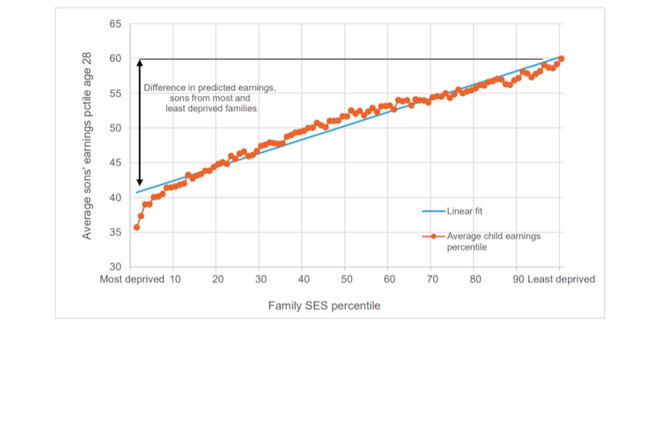
Figure 4.1 depicts the average earnings rank for children from each percentile of parents’ SES in the data (in orange) and the linear relationship we estimate (in blue) between parental socio-economic circumstances and sons’ rank in the earnings distribution at age 28, ranging from those who come from the most deprived families in childhood on the left to those who come from the least deprived families on the right of the figure. Each orange dot represents the average earning percentile at age 28 of sons born in a family at a particular percentile of the SES measure. The relationship is broadly linear (the points align along a fairly straight line), with the exception of the bottom five percentiles, where the relationship is more concave. This gives us confidence that our linear model (Equation 1 in Section 3) is broadly an appropriate way to describe the relationship between family circumstances and sons’ earnings.

If the relationship we estimate (the blue line in Figure 4.1) were flat, all sons would, on average, have the same earnings at age 28, regardless of their parental SES. The steeper this line is, the stronger the association between parental SES and adult earnings. For England overall, we find that, on average, sons from the least deprived families end up around 20 percentiles higher up the earnings distribution at age 28 than sons from the most deprived families (with the former earning on average £27,500 a year and the latter £13,200 a year at age 28).

Figure 4.1: Sons’ labour market earnings at age 28 by family circumstances at age 16 in England

Question 6

5.  Regional differences in intergenerational mobility

Accepted Answer

In this section, we report our estimates of mobility for each region in England, which we discuss in Section 1 of the main report. We again focus on two measures of mobility. Here, first, we show the average labour market earnings in early adulthood for children who were eligible for FSM at age 16 across local authorities, measuring how the life chances of disadvantaged sons vary across England. We then consider a measure of relative mobility, i.e. a measure of the differences in earnings for those sons from the most and the least deprived families within local authorities, capturing equality of opportunity within areas. We end the section with a description of the characteristics of areas that have high and low earnings outcomes for FSM sons, and areas that have high and low levels of relative mobility.

There were large differences in the pay of disadvantaged sons depending on where they grew up, both compared with disadvantaged sons from other areas and in terms of relative mobility, or the pay gaps between sons from the most and least deprived families. Areas with lower mobility are typically more deprived, with fewer ‘outstanding’ schools, and fewer professional and managerial jobs.

Earnings for sons eligible for FSM

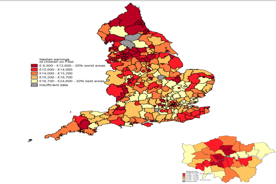
Figure 5.1 plots the median labour market earnings of those sons eligible for FSM in secondary school across all local authorities in England. The dark red areas are the 20% of local authorities where FSM-eligible sons have the lowest median earnings at age 28, while the lightest areas are the 20% of local authorities with the highest median earnings for FSM-eligible sons. The grey areas do not have sufficient numbers of sons eligible for FSM for us to compute these numbers reliably. The bottom map zooms in on the small London boroughs. Table 5.1 details some of the local authorities with the highest and lowest median earnings at age 28 for FSM-eligible sons.

While our national estimate showed that at the national level, the median earnings of those eligible for FSM was £13,500 at age 28, Figure 5.1 shows that this masks large differences in the median earnings of children from different areas. In Chiltern, for example, an area outside the M25 between High Wycombe and Watford, sons eligible for FSM at age 16 have median earnings of £6,900 a year at age 28, while similar groups in Uttlesford in Essex and Forest Heath in Suffolk have median earnings of over £21,000 a year at 28.

Differences in the earnings of sons who were disadvantaged at 16 do not follow the typical north/south divide. There are broad areas in the north west around Manchester, Sheffield and Leeds (dark red shading), and in the north east, where sons who grew up in those places and were disadvantaged at age 16 earned very little at age 28 (less than £10,000 in Gateshead, for example). But there are also broad areas in Kent and Sussex with low earnings for sons who grew up there and were disadvantaged at 16; in Hastings the average earnings at age 28 were £10,600 a year. There are also pockets in the west and south west of the country with low earnings for this group: in Malvern Hills just east of Wales, and in West Devon, sons who grew up there who were disadvantaged at age 16 earned less than £10,000 a year at age 28.

There are also large differences across local authorities that are close to each other. While many of the highest-earnings local authorities are around London, the story within London boroughs is mixed. While Havering, Barking, Newham, Tower Hamlets and Hillingdon are among the highest-earnings boroughs, Haringey, Islington, Wandsworth, Westminster, and Kensington and Chelsea are among the lowest-earnings boroughs for disadvantaged sons. There are also pockets of high-earnings local authorities across England. Disadvantaged sons at age 16 who grew up in South and East Staffordshire and those who grew up in South Ribble, just south of Preston, have median earnings of over £17,000 at age 28.

Table 5.1: Local authorities with highest and lowest median earnings at age 28 for sons eligible for Free School Meals

Local authorities with highest earnings – median earnings at 28 for FSM sons (£19,200 to £24,600)

Broxbourne
East Hertfordshire
Forest Heath
Havering
Reigate and Banstead
Spelthorne
Uttlesford
Welwyn Hatfield
West Oxfordshire
Wokingham

Local authorities with lowest earnings – median earnings at 28 for FSM sons (£6,900 to £10,400)

Bradford
Chiltern
Hartlepool
Hyndburn
Gateshead
Kensington and Chelsea
Malvern Hills
Nottingham
Sheffield
West Devon

Figure 5.1: Earnings at age 28 for disadvantaged sons at age 16, across local authorities in England where they grew up

Relative intergenerational mobility (pay gaps)

We now consider patterns in relative mobility across local authorities. Here, we are interested in the difference in earnings between sons from the most and least deprived families at age 16 growing up in the same region. To consider this, we use our measure of relative mobility in terms of rank in the earnings distribution and calculate it for each area. That is, we consistently rank sons within each area based on their rank in the national distribution of family advantage. This means that within each area we always compare the earnings of sons who are in the top 1% most advantaged families in the national distribution with sons who are the bottom 1% least advantaged families in the national distribution. Areas with the largest pay gaps are less mobile, offering less equal opportunities. Areas with smaller pay gaps are more mobile, offering more equal opportunities.

At the national level, sons from the least deprived families (who earned on average £27,500 a year) were 20 percentiles higher than sons from the most deprived families (who earned on average £13,200 a year). But this again masks large differences in the size of those gaps across local authorities (see Table 5.2 and Figure 5.2). The areas with the smallest pay gaps, of which the majority are Inner London boroughs, have differences of only 7 to 10 percentiles in the pay of sons from the most and least deprived families. In contrast, in the areas with the largest pay gaps – the least mobile areas, or those with the least equality of opportunity, such as Chiltern and Luton – there are large differences, of over 25 percentiles, between the pay of sons from the most and least deprived families. This is 2.5 times larger than the earnings gap found in those areas that offer the most equality of opportunity.

There are also large differences across local authorities within regions. As the smaller London map in Figure 5.2 shows, while Inner London boroughs feature heavily in the list of areas with the smallest pay gaps, there are areas of Outer London such as Bexley and Harrow which have large pay gaps (are among the least mobile), with differences between the earnings of the most and least deprived sons of 22 to 23 percentiles.^{[footnote 8]}

This pattern can be seen across the country in the larger map in Figure 5.2. In Manchester there is a 13-percentile pay gap between those from the most and least deprived families, while in neighbouring Bolton and Oldham the pay gap is 23 percentiles. In the south west, East Devon has a 13-percentile pay gap between sons from the most and least deprived families, while neighbouring Torbay has a 23-percentile pay gap. In Derbyshire, South Derbyshire has an 11-percentile pay gap while Derby has a 22-percentile pay gap between sons from the most and least deprived families. And in Yorkshire and the Humber, East Riding has a 16 percentile pay gap, while in Hull the gap is 25 percentiles.

Figure 5.2: Pay gaps at age 28 between the most and least deprived sons at age 16, across local authorities in England where they grew up

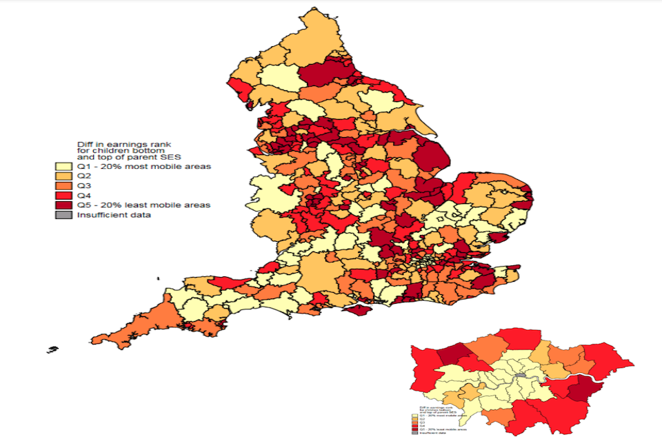
Table 5.2: Local authorities with the smallest and largest pay gaps at age 28 between the most and least deprived sons at age 16, by where they grew up

Local authorities with the smallest pay gaps (pay gap between the most and least deprived sons of 7 to 10 percentile points)

Kensington and Chelsea
Camden
Chichester
Hackney
Hammersmith and Fulham
Islington
North Dorset
Oxford
Southwark
Westminster

Local authorities with the largest pay gaps (pay gap between the most and least deprived sons of 24 to 28 percentile points)

Basildon
Bradford
Chiltern
Corby
Coventry
Hyndburn
Kingston upon Hull
Luton
North East Lincolnshire
Waveney

Table 5.3: Range of earnings rank differences in area for each quintile

Quintile	Range of earnings rank differences between most and least deprived sons
Q1 – most mobile areas	7 to 15 percentile points
Q2	15 to 17 percentile points
Q3	17 to 19 percentile points
Q4	19 to 21 percentile points
Q5 – least mobile areas	21 to 28 percentile points

What do areas with different levels of mobility look like?

We can use local area characteristics across local authorities to describe broad differences between areas with high and low earnings outcomes for FSM-eligible sons and between areas with small and large pay gaps between the most deprived and least deprived sons (areas with high or low relative mobility). These characteristics are measured around the time the sons in our sample were age 16. These are used to paint a picture of the areas with low and high levels of mobility for deprived sons, and should not be misinterpreted as necessarily driving these patterns of mobility.

The first columns of Table 5.4 show the characteristics of areas with low and high pay for disadvantaged sons, where we define areas with high (low) earnings outcomes as those that have earnings for FSM children above (below) the national mean (£13,500). At the time our cohorts were growing up in these areas, areas with lower earnings outcomes for FSM-eligible sons were typically more deprived, with around one third of local authorities in the bottom 20% of the IMD compared with around one in 20 high-mobility areas. This is consistent with other characteristics of these areas. Typically, areas with low earnings outcomes for FSM-eligible sons had lower proportions of individuals working in professional and managerial jobs, and higher proportions of inactivity. These areas were more densely populated and have lower median house prices. The proportion of ‘outstanding’ schools was lower in areas with lower earnings outcomes for FSM-eligible sons and infant health outcomes were worse, with higher rates of low birthweight and higher infant mortality rates compared with areas with high earnings outcomes for FSM- eligible sons.

Table 5.4: Local characteristics of areas with high and low earnings for disadvantaged sons, and high and low relative mobility

	High earnings	Low earnings	High relative mobility	Low relative mobility
Percent in lowest IMD quintile	4%	34%	7%	25%
Percent in professional job	29%	25%	29%	25%
Percent inactive	31%	35%	32%	33%
Percent ethnic minority	6%	9%	7%	7%
Population density (number of persons per hectare)	12	23	15	15
Median house prices	£99,000	£79,500	£100,400	£77,300
Percent ‘outstanding’schools	27%	22%	26%	23%
Percent low birthweight (<2.5kg)	7%	8%	7%	8%
Infant mortality rate / 1000	4.4	5.8	4.7	5.0

The last two columns of Table 5.4 present the average characteristics of more mobile areas (areas with relative mobility above the national rate) and less mobile areas (areas with relative mobility below the national rate). At the time our cohorts were growing up, areas with low levels of relative mobility were typically more deprived, with around a quarter of local authorities in the bottom 20% of the IMD compared with around one in ten areas of high relative mobility. Unlike for areas with lower and higher earnings outcomes for FSM-eligible sons, the share of people working in professional and managerial jobs, inactivity rates and population density were very similar across areas with low and high levels of relative mobility. There were larger differences in terms of median house prices, with lower-mobility areas having lower prices than high-mobility areas. As with our measures of earnings outcomes for FSM-eligible sons, areas with low relative mobility had a lower proportion of ‘outstanding’ schools. Areas of low relative mobility also had higher rates of low birthweight, although infant mortality rates were similar across areas.

Question 7

6.  The role of education in driving mobility at the national level

Accepted Answer

Much existing research on social mobility identifies education as playing a potentially important role in explaining intergenerational mobility, or the link between family circumstances and adult labour market earnings. Broadly speaking, this is because individuals from richer families typically do better at school, and this higher educational achievement is then rewarded in the labour market. In this section, we explore, first from a theoretical perspective, the channels through which education can account for part of the link between childhood circumstances and adult earnings. We then present estimates of the role of education in driving intergenerational mobility overall in England and discuss the importance of each channel separately.

How does education drive intergenerational (im)mobility?

Figure 6.1 shows the different pathways through which family circumstances affect adult labour market earnings, including education.

Figure 6.1: The role of education in transmitting incomes across generations

The first arrow depicts the link between family circumstances and educational achievement. In other words, it measures the size of differences in educational qualifications for those from the most deprived families compared with the least deprived families. These differences exist, for example, because richer families can afford to move closer to better schools (which tend to be in more expensive areas), and can provide a richer home learning environment or access to resources (e.g. private tuition) that enhance school achievement.

The second arrow depicts the link between educational achievement and adult labour market earnings. This relationship is often called the returns to education, and it measures how much more the top-performing pupils earn relative to the lowest-performing pupils.

Much empirical evidence suggests this relationship is strong. The higher the returns to education are, the stronger the mechanism through which educational inequalities between pupils from differences socio-economic backgrounds translates into earnings inequalities between them. The role that education plays overall in the transmission of socio-economic circumstances across generations therefore depends on the strength of both the first and the second arrow.

The third arrow depicts the extent to which family circumstances are related to adult labour market earnings for people with similar educational achievement levels (or conditional on educational achievement). This channel captures the fact that sons from more affluent families can have a direct labour market advantage, over and above educational achievement, for example through their access to better social networks or career opportunities and greater spatial mobility to seek out opportunities. It could also capture the fact that, relative to sons from more deprived families, sons from more affluent families have higher levels of skills unrelated to educational achievement that are rewarded in the labour market. This could include, for example, soft skills or self- confidence (to the extent that these do not affect educational achievement).

How much of the intergenerational transmission is through education?

Figure 6.2 shows that at the national level, for the cohort of sons that we study, 70% of the association between childhood circumstances and adult labour market earnings at age 28 can be accounted for by differences in educational achievement of the sons up to GCSE level.^{[footnote 9]} These results hold when measuring educational achievement using test scores at age 11, 16 and 18, participation at university, and university course metrics based on average labour market returns and selectivity of the course. The remaining 30% of the relationship remains unaccounted for by our measures of education, which could be picking up differences in subjects studied (we only measure total points score at age 16), unmeasured skills not related to education, and wider inequalities in the labour market that persist for people with similar levels of educational achievement, such as social networks, access to internships and broader cultural differences between people from different backgrounds (Friedman and Laurison, 2019).

Figure 6.2: Proportion of intergenerational transmission that works through educational qualifications

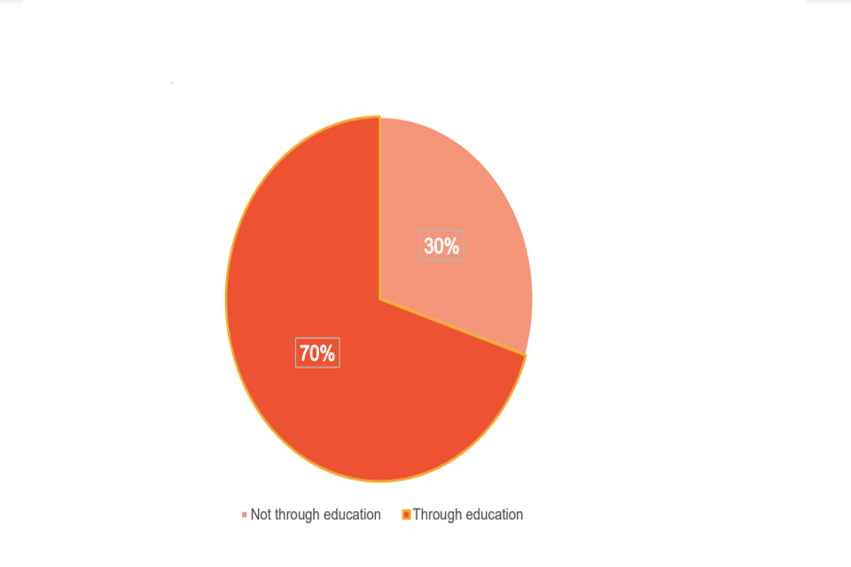
As illustrated in Figure 6.2, 70% of the transmission of circumstances across generations that works through educational attainment is composed of (1) the relationship between family circumstances in childhood and educational achievement; and (2) the differences in labour market earnings of those who do very well at school relative to those who perform relatively poorly.

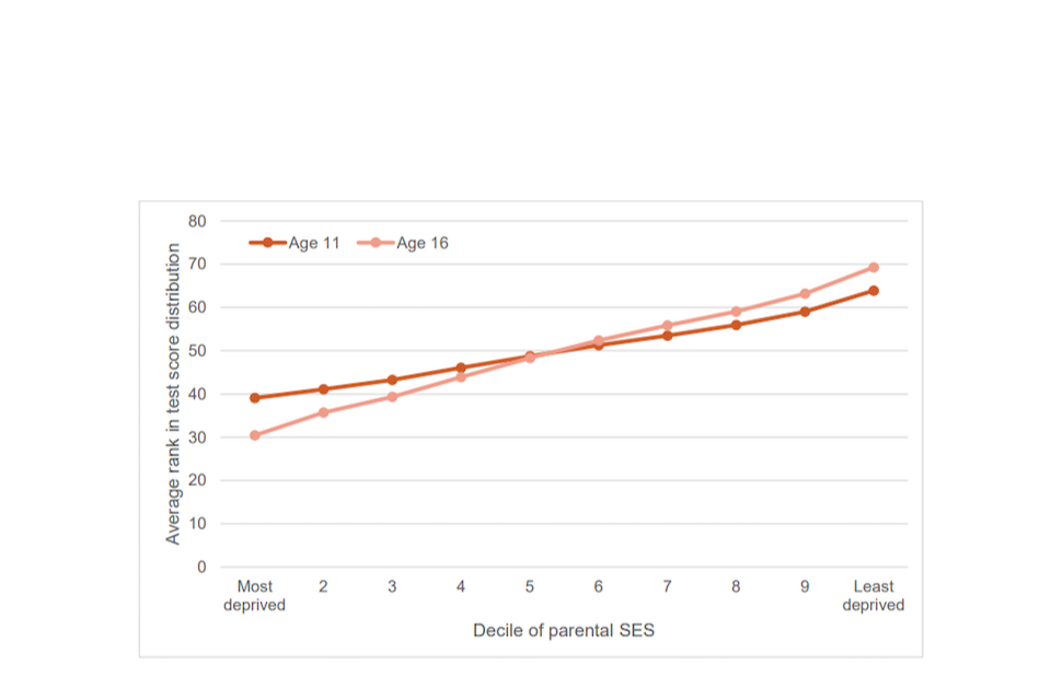
Figure 6.3 illustrates this relationship between family circumstances in childhood and educational achievement (the first arrow in Figure 6.1) across England, showing the average difference in educational achievement for those from the most deprived (left-hand side) and the least deprived (right-hand side) families. Comparing those from the most deprived families at age 11 first, if we were to rank everyone in the country in terms of their performance at age 11, they would be found at the 39th percentile on average, while the least deprived families would be found at the 64th percentile of educational achievement. There is therefore a 25-percentile difference in the average performance of sons from the most and least deprived groups of families at age 11.

Interestingly, this gap widens as children get older and is even more pronounced at age 16 (lighter line) than at age 11 (darker line). By age 16, if similarly rank everyone in the country in terms of their performance in their best eight GCSEs (or equivalents), those from the most deprived 10% of families perform on average at the 30th percentile – equivalent to a pupil achieving three D, four E and one F grade – while those from the least deprived 10% of families perform at the 69th percentile – equivalent to a pupil achieving one A, three B and four C grades – of educational achievement. The difference or gap in performance at age 16 between the most and least deprived families is 39 percentiles at age 16.

Figure 6.3: Educational achievement by family circumstances at age 11 and age 16 in England

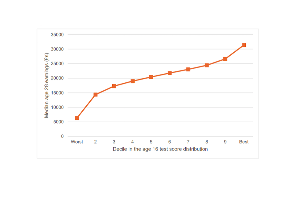
As discussed earlier in the section, the way these differences in educational achievement by age 16 translate into differences in adult earnings in the labour market depends on the returns to education in the labour market (or the strength of the link between educational achievement and earnings). Figure 6.4 shows the differences in labour market earnings of those who do very well at school relative to those who perform relatively poorly (the second arrow in Figure 6.1) across England. Here we illustrate the average labour market earnings of those who are the lowest performers at age 16 (left-hand side) – achieving equivalent to one F at GCSE – up to those who are the highest performers at age 16 (right-hand side) – achieving equivalent to three A*s, three As, and two Bs at GCSE. The poorest performers in terms of GCSE achievement are paid on average £6,300 a year at age 28, while the highest performers are paid on average around five times as much (£31,400 a year). If we rank sons into percentiles, this is equivalent to those in the lowest percentile of test scores being 41 percentiles lower than those in the highest percentile of test scores in the age 28 earnings distribution.

Together, these two channels – (1) sons from less deprived backgrounds have better educational attainment, and (2) better educational attainment leads to higher adult earnings – explain 70% of the persistence between family circumstances and adult earnings that we find overall in England. This evidence is in line with previous research (Blanden, Gregg and Macmillan et al., 2007) which finds a substantial role for education in driving intergenerational (im)mobility across the country.

Figure 6.4: Labour market earnings at age 28 by educational achievement at age 16 in England

Question 8

7.  The role of education in explaining differences in mobility

Accepted Answer

The previous section has shown that at the national level, a large portion of the link between adult earnings and family circumstances can be traced back to differences in educational attainment across sons with different family circumstances. But the fact that educational achievement is an important driver of differences in opportunities between sons everywhere does not necessarily mean that it explains why we see differences in opportunities across areas.

For education to explain regional differences in intergenerational mobility, there need to be: (1) regional differences in educational gaps between sons from the most deprived and the least deprived families, such that the areas with the highest pay gaps are also those with the highest education gap; and/or (2) regional differences in the returns to education, such that the regions with the highest pay gaps are also those with the highest returns. In other words, the strength of the first and second arrow in Figure 6.1 needs to vary across areas in England in ways that parallel the regional differences in intergenerational mobility observed in Figure 5.1. Importantly, this variation also needs to be large enough to account for the large differences in earnings gaps by SES across areas.

In this section, we empirically assess the role of education in driving the geographic differences in intergenerational mobility that we observe across areas (Figure 5.1). Mirroring the analysis in Section 6, we first investigate how educational gaps between the most and least deprived sons vary across areas. We then turn to analysing how the returns to education (or the earnings gaps between sons with high and low educational achievement) vary across areas. We then combine these two paths, to show the total contribution of education in accounting for the intergenerational transmission across areas.

We find large achievement gaps between sons from the most and least deprived families across areas, and differences in the earnings outcomes of the lowest- and highest- achieving sons by place. Interestingly, when we combine these two channels, education makes a broadly stable contribution to explaining mobility rates across areas – it still accounts for the majority of the SES-to-earnings transmission within each place (on average 80%) – but does not account for differences in this transmission across places. Instead, it is differences in the direct association between parental SES and sons’ earnings, comparing sons with similar educational achievement (channel 3 from Figure 6.1), that explain differences in mobility rates across areas.

How do educational gaps between the most and least deprived sons vary across areas?

Figure 7.1 and Table 7.1 show that there are large differences in educational achievement among the most and least deprived sons across areas. As with earnings gaps, there are notable differences in educational achievement gaps across local areas within regions. In North Dorset, for example, there is a 37-percentile difference between the education outcomes of the most and least deprived sons, compared with 48-percentile differences in Poole and Bournemouth. Similarly, in Manchester the difference is 37 percentiles, compared with 48 in Trafford. And on the North Yorkshire coast, East Riding has a 39- percentile difference in the education outcomes of the most and least deprived children, compared with 49 percentiles in Scarborough.

The London map of Figure 7.1 illustrates that many of the Outer London boroughs have larger differences in educational outcomes between the most and least deprived children: in Richmond there is a 48-percentile difference while in neighbouring Wandsworth the difference is only 28 percentiles. The areas with the smallest differences in education outcomes between the most and least deprived children all tend to be Inner London boroughs. Here the gaps in education outcomes are about a third to half the size of those in the local authorities with the highest gaps in the age 16 education outcomes for the most and the least deprived children. In contrast, the boroughs with the largest SES gaps in KS4 performance have over 50 percentiles’ difference in the GCSE performance of the most and least deprived sons.

Interestingly, while patterns of education gaps (Figure 7.1) have some similarities with patterns in pay gaps across areas (Figure 5.1), most notably in Inner London, there are also some clear differences across England: the places with the largest pay gaps between the most and least deprived sons are not necessarily the places with the largest gaps in educational achievement among the most and least deprived sons across areas. More precisely, half of these local authorities also have large pay gaps between the most and least deprived sons, but the other half have smaller pay gaps.

Figure 7.1: Differences in age 16 education percentiles between sons from the most and least deprived families, across local authorities in England

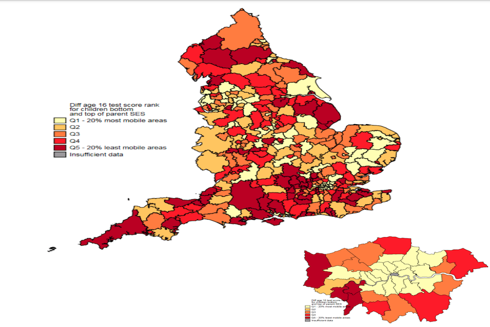
Table 7.1: Local authorities with largest and smallest educational gaps between the most and least deprived sons at age 16, by where they grew up

Local authorities with the smallest education gaps (education gaps between the most and least deprived sons of 19 to 28 percentiles)

Camden
Hackney
Hammersmith and Fulham
Islington
Kensington and Chelsea
Lambeth
Southwark
Tower Hamlets
Wandsworth
Westminster

Local authorities with the largest education gaps (education gaps between the most and least deprived sons of 51 to 57 percentile points)

Chiltern
East Lindsey
Epson and Ewell
Lancaster
Lewes
Oxford
South Bucks
Torbay
Windsor and Maidenhead
Wycombe

Table 7.2: Range of gaps in age 16 test score rank in area for each quintile

Quintile	Range of earnings rank differences between most and least deprived sons
Q1 – smallest gaps	19 to 40 percentile points
Q2	40 to 42 percentile points
Q3	42 to 45 percentile points
Q4	45 to 47 percentile points
Q5 – largest gaps	47 to 57 percentile points

What do areas with large educational gaps between the most and least deprived sons look like?

Table 7.3 reports the average characteristics of areas with larger and smaller differences in relative education outcomes compared with the national average. Specifically, areas with small (large) education gaps are the areas where the difference in educational outcome rank between sons of the most and least deprived families is below (above) the national average (39 percentiles).

Areas with large education gaps are less deprived, less densely populated and less ethnically diverse, relative to areas with small education gaps between sons from the most and least deprived families. While areas with larger education gaps have a similar proportion of outstanding schools, and similar rates of participation at 16 to 18 and in higher education, to areas with smaller education gaps, they have greater segregation in terms of both achievement and SES, and are far more likely to have grammar schools (secondary school selection based on an entry test at age 11) in the area. Of the 10 local authorities with the largest education gaps between the most and least deprived children, seven are areas that have grammar schools (Lewes, Windsor and Oxford do not). Southend-on-Sea and Tunbridge Wells, also grammar school areas, are also among those with the largest gaps.

Table 7.3: Local characteristics of areas with smaller and larger gaps between the educational achievement of the most and least deprived sons

	Small education gaps	Large education gaps
Percent in lowest IMD quintile	22%	11%
Percent ethnic minority	14%	5%
Population density (number of persons per hectare)	34	12
Percent ‘outstanding’ schools	25%	25%
Percent post-16 participation	40%	42%
Percent post-18 participation	35%	33%
Percent of KS4 test score variation in area between schools	17%	22%
Percent of SES variation in area between schools	18%	21%
Percent of LAs with grammar schools	8%	21%

Earnings differences for high- and low-achieving sons

Figure 6.4 highlighted differences in the earnings outcomes of high and low achievers at the national level. If we rank sons according to their achievement at age 16, the highest- achieving sons’ earnings were 36 percentiles higher than those of the lowest-achieving sons. Figure 7.2 and Table 7.4 show how these earnings differences for high- and low- achieving sons vary across each area in England.

In the local authorities with the highest pay gaps by sons’ achievement at age 16, such as Eden in Cumbria, Oxford, West Oxfordshire and Ryedale in North Yorkshire, the difference in earnings percentiles between the highest- and lowest-achieving sons in age 16 tests is around 22 to 26 percentiles. These areas also tend to have relative mobility rates above the national average. The local authorities with smaller pay gaps between high- and low- achieving sons (lower returns to education), such as Rochford in Essex, Copeland in Cumbria, Mansfield in Nottinghamshire and Luton, have differences in age 28 earnings percentiles for the highest- and lowest-achieving sons at age 16 of around 40 percentiles. Most of these local authorities also have relative mobility rates below the national average.

Figure 7.2: Differences in labour market earnings at age 28 between the highest- and lowest-achieving sons at age 16, across local authorities in England

Table 7.4: Local authorities with the largest and smallest earnings gaps between the highest- and lowest-achieving sons at age 16, across England

Local authorities with smallest pay gap (earnings gaps between the highest and lowest achieving sons of 22 to 27 percentiles)

Derbyshire Dales
Eden
High Peak
Mid Devon
Oxford
Ryedale
South Lakeland
Teignbridge
Torridge
West Oxfordshire

Local authorities with largest pay gap (earnings gaps between the highest and lowest achieving sons of 40 to 42 percentiles)

Copeland
Dudley
Luton
Mansfield
Nottingham
Rochford
Sandwell
Stockton-on-Tees
Warrington
Wigan

Table 7.5: Range of earnings rank differences in area for each quintile

Quintile	Range of earnings rank differences between highest and lowest attaining sons at age 16
Q1 – smallest gap	22 to 31 percentile points
Q2	31 to 33 percentile points
Q3	33 to 35 percentile points
Q4	35 to 37 percentile points
Q5 – largest gap	37 to 42 percentile points

What do areas with large earnings gaps between high- and low- achieving sons look like?

Table 7.6 reports the average characteristics of areas with small and large earnings gaps between high- and low-achieving sons at age 16. The pattern of differences between these two types of areas is strikingly different from that seen in previous figures. Most notably, we see an urban–rural divide, with most cities having relatively large earnings differences between children with the highest and lowest KS4 performance, while this gap is much smaller in rural areas. Areas with larger earnings gaps between high- and low-achieving sons at age 16 are also more deprived than those with small differences in earnings. They have a lower proportion of professional and managerial jobs and higher rates of inactivity. They are more ethnically diverse and more densely populated, with lower median house prices.

Table 7.6: Characteristics of areas with small and large returns to educational achievement at age 16

	Smaller returns to education	Larger returns to education
Percent in lowest IMD quintile	4%	31%
Percent in professional job	29%	26%
Percent inactive	31%	34%
Percent ethnic minority	4%	11%
Population density (number of persons per hectare)	11	24
Median house prices	£98,000	£82,700

To what extent does education drive regional differences in intergenerational mobility in England?

The evidence so far presented in this section suggests that, while education is likely to play a role in explaining intergenerational mobility, it is not obvious that education explains the patterns of regional differences in earnings gaps between the most and least deprived sons that we presented in Section 5. Indeed, while there are regional differences in educational gaps between the most and least deprived sons across areas, the patterns do not map onto regional differences in pay gaps in a ubiquitous way. Areas with large educational gaps are not always areas with large earnings gaps between the most and least deprived sons. Moreover, while there is some regional variation in the returns to education, areas with high returns are far from mapping directly onto areas with the largest earnings gaps between the most and least deprived sons. Crucially, when we combine these two channels, these differences are also not large enough to account for the variation in SES-to-earnings transmission across areas.

Figure 7.3: Relative contribution of education and wider labour market factors to differences in intergenerational mobility across England

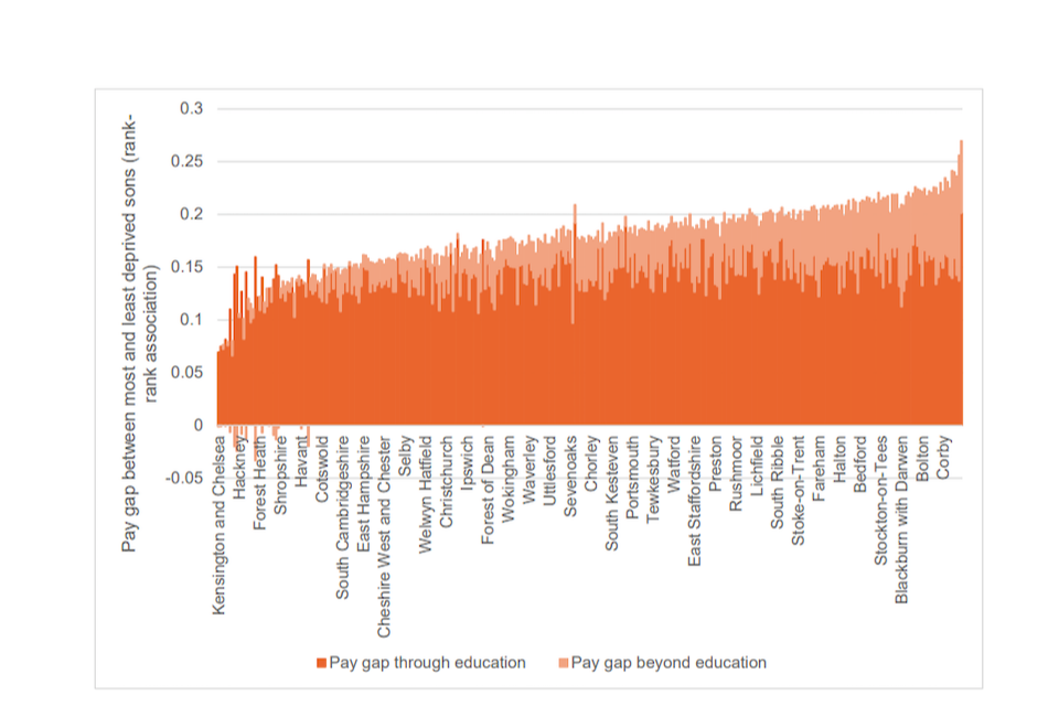
Figure 7.3 illustrates the pay gap for every area in England, from the most mobile (smallest gaps) on the left to the least mobile (largest gaps) on the right. The dark orange portion of the bar shows the part of the pay gap that is explained by the total educational differences between sons from the most and least deprived families (educational achievement differences for the most and least deprived sons, arrow 1 in Figure 6.1, multiplied by earnings differences for low and high achievers, arrow 2 in Figure 6.1). The light orange portion shows the part of the pay gap that remains even when comparing sons with the same educational achievement. Figure 7.3 clearly shows that education explains the majority of the pay gap (or total mobility) in every area of England – around 80% on average. The main differences across areas are working through the light orange portion of the bar – the pay gap that exists even when comparing sons with similar educational achievement. This pattern holds when we compare sons with the same achievement at age 11, 16 and 18, and attending an equally selective university course. This is similar to the findings of Gregg et al. (2017) when comparing two low-mobility countries (the US and Britain) with a higher-mobility country (Sweden).

To show this another way, we can compare the pay gaps of the most and least deprived sons with the same education across England. In other words, we estimate the importance of the third arrow in Figure 6.1, which represents the role of family socio-economic circumstances in driving earnings beyond education. Figure 7.4 depicts the strength of this relationship for each area in England. This shows a strikingly similar pattern across areas to that found in Section 5 (Figure 5.2).

This suggests that the main reasons for differences in social mobility (or the size of the pay gaps of sons from the most and least deprived families) across areas are found beyond education, in the labour market. In the least mobile areas, family background casts a long shadow, predicting labour market success regardless of the education that sons achieve. This could be through richer sons having better social networks and greater access to career opportunities.^{[footnote 10]} In more mobile areas, educational achievement alone predicts labour market success – family background has no lasting influence.

What might be driving this lasting effect of family background in the most unequal areas? While it is hard to explore further explanations in our data, we know that this group of sons were either entering, or establishing themselves in, the labour market as the Great Recession took hold. We know that these areas with the most unequal opportunities are more deprived and have fewer labour market opportunities in terms of the proportion of people working in professional and managerial jobs. We also know from other research that sons from the most deprived families are disproportionately impacted by bad labour markets (List and Rasul, 2011; Gregg and Tominey, 2005; Macmillan, 2014). A possible explanation, then, is that sons from more advantaged families are better placed to navigate the restricted opportunities available in unequal areas, either by moving out of these areas or by utilising their family networks to gain an advantage in accessing the limited options within them.

Figure 7.4: Differences in earnings rank between the most and least deprived sons at age 16 controlling for education, across local authorities in England

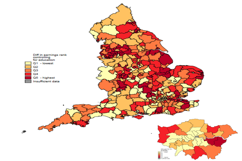
Table 7.7: Range of earnings rank differences in area for each quintile

Quintile	Range of earnings rank differences between most and least deprived sons controlling for education
Q1 – smallest differences**	−3 to 2 percentile points
Q2	2 to 3 percentile points
Q3	3 to 4 percentile points
Q4	4 to 5 percentile points
Q5 – highest differences	5 to 12 percentile points

Question 9

8.  Policy challenges

Accepted Answer

In this report we have shown large differences in the pay of disadvantaged sons based on where they grew up, and large differences in the pay gaps between these sons and their counterparts from more affluent families who grew up in the same area. We have also shown that while education gaps between the most and least disadvantaged sons account for a large part of the pay gaps found throughout the country, they cannot explain the differences in pay gaps between places. In other words, if we were to equalise educational outcomes between sons of the poorest and richest families in each area, gaps in earnings outcomes would be significantly reduced but the differences in pay gaps between local authorities would remain. To equalise opportunities for those from the most and least deprived backgrounds, then, educational policies will be crucial. But in order to ‘level up’ between places, these need to be supplemented with wider-ranging policy interventions such as labour-market-focused interventions.

The importance of education in social mobility has been widely recognised, and many initiatives are attempting to reduce educational inequalities, but in order to create a truly socially mobile country, it will also be important to understand what barriers prevent equally achieving deprived sons from succeeding in the labour market in certain areas of the country. These findings further raise the questions of which areas policy-makers should focus on and how existing policy ties in with the findings of this report. In this section, we discuss the answers this research is able to provide to these questions and highlight areas where further investigation and data are needed to answer them fully.

Barriers to equal achievement in the labour market

Figure 7.3 illustrated the key finding that while education can explain a large part of the pay gap nationally, it does not explain the differences in pay gaps across local authorities. This finding provides a challenge to the notion that educational investment alone will remove differences between areas. Education gaps account for the majority of the pay gaps in all areas, and reducing these is important in and of itself. However, we also need to look at equalising the labour market opportunities that are available for young people with the same education level from poor and richer backgrounds if we are to ‘level up’ between places. Beginning to tackle this gap requires us to understand what drives it – only then can we design effective interventions that address the specific roots of intergenerational disadvantage.

While the current report does not allow us to disentangle the drivers of this gap, we highlight here several potential channels through which family disadvantage may have an impact on earnings, over and above educational attainment which previous research has focused on. More research will be needed to determine the relative importance of each of these channels, and indeed of others not mentioned here.

First, sons from deprived backgrounds may lack family connections which help with learning about, and accessing, good jobs. These inequalities in social capital could be exacerbated by sons from deprived families having poorer soft skills. Poorer soft skills may put individuals at a disadvantage when it comes to networking, interviews and ultimately securing well-paid jobs. As shown in Section 1 of the main report, the least mobile areas are also those with fewer high-skilled jobs, so those skills and connections may be particularly valuable in enabling access to the few good jobs available in these areas. Increasing the number of available skilled jobs (see the discussion of the Towns Fund in the final part of this section) could be another channel through which sons from deprived background might be more able to access good jobs.

Second, differences between the schools attended by pupils from different socio-economic backgrounds may play a role alongside individual differences in social capital and non- academic skills. We showed in the main report that sons from deprived areas were less likely to attend ‘outstanding’ schools. State schools in these deprived areas may also have fewer resources to spend on enrichment and career development activities, thereby equipping their students less well to succeed in the labour market.

Third, sons from deprived backgrounds may lack the financial capital available to more affluent sons to explore various job opportunities in the early stage of their career. A recent book by sociologists Sam Friedman and Daniel Laurison (2019) describes this factor as ‘the Bank of Mum and Dad’, and outlines various benefits to having the financial backing of parents at a precarious time in children’s careers, such as the ability to take unpaid internships.

Fourth, sons from deprived backgrounds may face higher costs to moving out of areas with limited opportunities relative to their peers from more affluent backgrounds, making them less able to seek out good opportunities elsewhere. The recent SMC report ‘Moving out to move on’ suggests that this role could be significant – it finds that not only are more deprived sons less geographically mobile, but when individuals from deprived areas (which we find to also have the lowest social mobility) do move, it is mainly towards other deprived areas.

Fifth, employers may have recruitment and retention policies in place that favour sons from more advantaged backgrounds in particular areas. Employers may advertise vacancies selectively, through either school or professional networks that are disproportionally accessed by more advantaged pupils. Particular recruitment practices may be disadvantageous to, or discriminate against, deprived individuals. Studying where, in the recruitment process of large firms, individuals from poorer backgrounds fail to progress is an important step towards understanding how employers’ recruitment policies can be made more inclusive. There may also be barriers to retention and progression within firms for those from the most deprived families. For example, Friedman and Laurison’s book highlights sponsorship by senior leaders that fast-tracks the careers of junior protégés with a ‘class-cultural affinity’ as one of the potential mechanisms. This observed difference in cultural capital could be allowing those from more advantaged backgrounds to get further in a firm than their disadvantaged counterparts.

Which areas should policy-makers focus on?

Our research has shown wide disparities in the adult experiences of deprived sons depending on where they were born – in terms of their earnings outcomes and in terms of how they fare relative to more affluent sons from the same place. This strongly suggests the need for place-based policies, and an important question for policy-makers when designing policies aimed at improving social mobility is who to focus on, or at least who to focus on first.

While we ideally strive for both higher pay for disadvantaged sons and smaller pay gaps between them and sons from more affluent families, how useful are small pay gaps if pay is low for all? Similarly, how promising is higher pay for the most disadvantaged sons, if the pay gap between them and the least deprived is large? Ultimately, the answer to these questions will depend on policy-makers’ and society’s objectives, but the research we have conducted can help identify areas that are in dire need of support because they offer both very poor and very unequal opportunities to disadvantaged sons.

To understand the multiple issues faced by each area, we consider both of our metrics together (Table 8.1). Over half of English local authorities have higher pay for disadvantaged sons and more equal opportunities compared with the national rates (column a). The remaining half are split evenly between areas with higher pay for disadvantaged sons but less equal opportunities; areas with more equal opportunities but lower pay for this group; and areas with less equal opportunities and lower pay for disadvantaged sons combined.

Areas with higher pay for disadvantaged sons chances but less equal opportunities (column b) have similar characteristics to those areas with higher pay and more equal opportunities: they have similarly low levels of deprivation, a similar population density, and similar education and labour market opportunities.

Areas with lower pay for disadvantaged sons but more equal opportunities (column c) look demographically different from those with higher pay for disadvantaged sons: they are more deprived and more densely populated, but they have similar levels of education and labour market opportunities.

But those areas with low pay for disadvantaged sons and less equal opportunities (column d) are very different in terms of demographics, education and labour market opportunities. These areas are very deprived, have moderate population density, and have starkly lower education and labour market opportunities, with far fewer ‘outstanding’ schools and far fewer professional occupations than the other areas. By combining metrics on pay for the most disadvantaged and equality of opportunities, then, we can see a particular group of big towns and smaller cities that offer very little opportunity for anyone, but particularly for the most deprived sons.

Table 8.1: Local characteristics of areas with a combination of high and low earnings for disadvantaged sons and high and low relative mobility rates (pay gaps)

	(a) high earnings, high relative mobility (small pay gaps)	(b) high earnings, low relative mobility (large pay gaps)	(c) low earnings, high relative mobility (small pay gaps)	(d) low earnings, low relative mobility (large pay gaps)
Proportion of local authorities	52%	17%	16%	15%
Percent in lowest IMD quintile	3%	5%	22%	46%
Percent in professional job	29%	28%	29%	21%
Percent inactive	31%	31%	34%	36%
Percent ethnic minority	6%	6%	10%	7%
Population density (number of persons per hectare)	11	13	29	17
Median house prices	£99,600	£97,000	£102,900	£55,600
Percent ‘outstanding’ schools	27%	27%	26%	18%
Percent low birthweight (<2.5kg)	6.8%	6.9%	7.4%	8.3%
Infant mortality rate / 1000	4.4	4.4	5.8	5.7

How does the current policy landscape tie in?

A recent policy initiative has recognised the limited opportunities available in towns relative to larger cities. The Towns Fund prospectus highlights that while successive governments have focused on cities as engines of economic growth, many struggling towns do not have the resources to build a strong local economy. The Towns Fund is therefore a promising initiative designed to use public investment, through Town Deals, to create the right conditions to encourage private investment through improving transport, labour force skills, and housing and commercial land availability.^{[footnote 11]} But the recent monitoring report from the SMC has highlighted areas of improvement for this scheme, including the need for more transparency in how places are selected into the scheme and how the programme will be evaluated.^{[footnote 12]}

There are 17 of the 50 LAs with low pay for disadvantaged sons and less equal opportunities named in the list of an initial 100 Town Deals across England, including Bolton, Dudley, Hastings, Rochdale, St Helens and Wolverhampton. But many of the other LAs, including smaller cities such as Stoke, Hull, Bradford, Leicester and Coventry, do not qualify. While Local Enterprise Partnerships (LEPs) play a key role at a more aggregate level in contributing to local economic strategies, the variation in pay and pay gaps within local areas suggests that this localised approach is an effective way of ensuring that funds are targeted where they are most needed.

Further, a recent place-based initiative focused on improving social mobility in specific areas – Opportunity Areas^{[footnote 13]} – targeted 12 local authorities that were defined as ‘challenging’, with multiple disadvantages across the life course. These areas received targeted investment (£72 million over three years) to provide tailored interventions, primarily to young people, to address stubborn local challenges and create ‘sustainable, long-term change’. The metric used to short-list candidates for this investment, the Social Mobility Index, combined information on area-level early years provision; the school performance of disadvantaged pupils; post-compulsory education and employment rates of disadvantaged pupils; and labour market indicators including pay, house prices, professional occupations and home ownership.^{[footnote 14]}

We find that 9 of the 12 Opportunity Areas fall into our column d group, offering both lower pay for disadvantaged sons and less equal opportunities. The three which do not fall into this group – Norwich, Ipswich and West Somerset – have poor education outcomes for disadvantaged sons but relatively good earnings outcomes. For example, both Ipswich and West Somerset have higher pay for disadvantaged sons and more equal opportunities, putting them firmly in column a of Table 8.1. Norwich has lower life chances for disadvantaged sons but has more equal opportunities in the form of small pay gaps between the most and least deprived sons (column c).

If effective, the interventions put in place within Opportunity Areas have the potential to reduce educational disadvantage in areas with the poorest and least equal opportunities for deprived individuals. This would already be an important achievement in reducing part of the disadvantage gap in those areas. The move towards increasing public investment to encourage private investment in towns through the Towns Fund is a further promising intervention, given that our analysis identifies a group of towns that offer the lowest pay for disadvantaged sons and the least equal opportunities between the most and least deprived sons. But an education-focused programme or a labour-market-focused programme alone is unlikely to be as effective as one which draws together multiple departments for a life-course-based approach to creating opportunities.

There is also a significant risk that existing interventions are likely to be dwarfed by the impact of the post-COVID-19 recession. Current estimates suggest this is likely to be the largest recession in history, and far deeper than the Great Recession that our cohort of sons experienced. If the lack of labour market opportunities reinforces the importance of family background, we might expect to see growing inequalities across the country. There is an urgent need to widen the scope of this research to further investigate the labour market barriers that exist for today’s young people from deprived backgrounds and implement interventions that can effectively protect them from the disproportionate impact of these recessions.

Next steps for research

While it is beyond the scope of this report to investigate the relative importance of these factors in driving regional differences in social mobility in England, it is imperative that further research is done to help policy-makers prioritise investments in interventions to reduce any remaining earnings gaps by socio-economic background for sons with the same education. While the current LEO dataset has been a step change in the available data to enable researchers to investigate social mobility differences across the country, there are three main improvements to the LEO dataset which would hugely benefit future research in this area and provide important further insights for policy-makers.

A first limitation of the current data is that it does not enable researchers to address the contribution of internal migration – and especially socio-economic differences in internal migration – to the regional differences in earnings gaps we unveiled in this analysis. This is because our data contain information only on where individuals grew up and not on where they live as adults. Adding this information (which is available in tax records) to the LEO dataset is a priority to enable further investigation of the role that internal migration, and differences in geographic mobility, play in explaining the patterns of social mobility we uncovered. As discussed above, previous work suggests that this role may be significant.

A second limitation of the current data is that we can only measure differences in opportunities for men in England. This is because (1) we cannot observe non-earned income or hours worked, and women from disadvantaged backgrounds are more likely to work part-time at the age we observe (28), and (2) linked administrative data records are currently only available in England. While we understand that hours of work are not available in administrative records, bringing in non-earned income, such as benefit income, and creating identifying variables that allow us to adequately link individuals in households, would allow researchers to measure total family income, thereby bringing women into the picture and giving a richer measure of family resources. Creating similar data linkages in the other home nations would allow for this research to be conducted across the whole of the UK.

Finally, the lack of linkage between parents and children does not currently allow researchers to measure parental income in childhood, thereby restricting them to using proxies of income such as measures of family deprivation based on FSM eligibility and local area deprivation, as used in this report. While other evidence has found this metric to be a promising proxy for permanent family income in longitudinal cohort studies (Jerrim, 2020) creating identifying variables that link between generations would allow for a richer picture of childhood circumstances. This would allow, for example, further investigation into the ages in childhood at which family deprivation is particularly detrimental to a child’s future outcomes.

We would encourage government departments across all home nations to build this type of data linkage into their future plans. This type of linkage is available in, for example, Scandinavian registry data, and much could be learnt from their approach to data linkage and their support of research using this data, which ultimately gives policy-makers the tools to design and enact better policy.

Question 10

References

Accepted Answer

Andrews, D. and A. Leigh. (2009). ‘More inequality, less social mobility’. Applied economics letters, 16(15): 1489-1492.

Araujo, M.C., P. Carneiro, Y. Cruz-Aguayo, N. Schady. (2017). ‘Teacher Quality and Learning Outcomes in Kindergarten’. The Quarterly Journal of Economics, 131(3):1415- 1453.

Belfield, C., J. Britton, F. Buscha, L. Dearden, M. Dickson, L. can der Eerve, L. Sibieta, A. Vignoesl, I. Walker and Y. Zhu (2018). ‘The relative labour market returns to different degrees’. Department for Education/Institute for Fiscal Studies Research Report https://assets.publishing.service.gov.uk/government/uploads/system/uploads/attachment_ data/file/714517/The_relative_labour_market-returns_to_different_degrees.pdf

Britton, J. and L. Dearden. (2015). ‘The 16 to 19 bursary fund: impact evaluation’. Department for Education Research Report. https://dera.ioe.ac.uk/33214/1/RR414_-_The_16_to_19_Bursary_Fund Impact_Evaluation.pdf

Bell, B., J. Blundell and S. Machin (2018). ‘The changing geography of intergenerational mobility’. CEP Discussion Paper No 1591.

Björklund, A. and M. Jäntti (2009). ‘Intergenerational income mobility and the role of family background’. Oxford handbook of economic inequality, 491: 521.

Björklund, A. and K. Salvanes (2010). ‘Education and family background: Mechanisms and policies.’ IZA Discussion Paper no. 5002.

Björklund, A., M. Jäntti and G. Solon (2005). ‘Influences of nature and 80 nurture on earnings variation: A report on a study of various sibling types in Sweden’, in S. Bowles, H. Gintis and M. Osborne Groves (eds), Unequal chances: Family background and economic success. Princeton, NJ: Princeton University Press, pp. 145–164.

Björklund, A., M. Lindahl and E. Plug (2006). ‘The origins of intergenerational associations: Lessons from Swedish adoption data’. Quarterly Journal of Economics 121: 999–1028.

Björklund, A., T. Eriksson, M. Jäntti, O. Raaum and E. Österbacka (2002). ‘Brother correlations in earnings in Denmark, Finland, Norway and Sweden compared to the United States’. Journal of Population Economics 15: 757–772. B.

Black, S. and P. Devereux (2011). ‘Recent developments in intergenerational mobility’, in O. Ashenfelter and D. Card (eds), Handbook of labor economics, Volume 4b. Amsterdam: North Holland Press, Elsevier.

Black, S., P. Devereux and K. Salvanes (2005). ‘Why the apple doesn’t fall far: Understanding intergenerational transmission of human capital’. American Economic Review 95: 437–449.

Blanden, J. (2013). ‘Cross-country rankings in intergenerational mobility: A comparison of approaches from economics and sociology’. Journal of Economic Surveys 27(1): 38–73.

Blanden J. and P. Gregg (2004). ‘Family income and educational attainment: A review of approaches and evidence for Britain’. Oxford Review of Economic Policy 20(2): 245–263.

Blanden, J. and L. Macmillan (2016). ‘Educational inequality, educational expansion and intergenerational mobility’. Journal of Social Policy 45(04): 589–614.

Blanden J, P. Gregg and L. Macmillan (2007). ‘Accounting for intergenerational income persistence: Noncognitive skills, ability and education’. The Economic Journal 117(519): C43–C60.

Blanden, J., A. Goodman, P. Gregg and S. Machin (2004). ‘Changes in intergenerational mobility in Britain’, in M. Corak (ed.), Generational income mobility. Cambridge: Cambridge University Press.

Bovenberg, L.A. and B. Jacobs (2005). ‘Redistribution and education subsidies are Siamese twins’. Journal of Public Economics 89: 2005–2035.

Carneiro, P., S. Cattan, E. Risa, S. Krutikova and K. Salvanes (2019). ‘Intergenerational mobility over time and across regions in Norway’. Mimeo.

Carneiro, P., I. Garcia, K. Salvanes and E. Tominey (2015). ‘Intergenerational mobility and the timing of parental income’. CEMMAP Working Paper, CWP66/15.

Chetty, R., J. Friedman, and J. Rockoff (2014). ‘Measuring the Impacts of Teachers: Evaluating Bias in Teacher Value-Added Estimates’. American Economic Review, 104(9): 2593-2632.

Chetty, R., D. Grusky, M. Hell, N. Hendren, R. Mandura and J. Narang (2017). ‘The fading American dream: Trends in absolute income mobility since 1940’. Science 356: 398–406.

Chetty, R. and N. Hendren (2018a). ‘The impacts of neighborhoods on intergenerational mobility I: Childhood exposure effects’. The Quarterly Journal of Economics 133(3): 1107– 1162.

Chetty, R. and N. Hendren (2018b). ‘The impacts of neighborhoods on intergenerational mobility II: County level estimates’. The Quarterly Journal of Economics 133(3): 1163–1228.

Chetty, R., N. Hendren, P. Kline and E. Saez (2014). ‘Where is the land of opportunity? The geography of intergenerational mobility in the United States’. The Quarterly Journal of Economics 129(4): 1553–1923.

Chowdry, H., C. Crawford, L. Dearden, A. Goodman and A. Vignoles (2013). ‘Widening participation in higher education: Analysis using linked administrative data’. Journal of the Royal Statistical Society A 176(2): 431–457.

Corak, M. (2006). ‘Do Poor Children Become Poor Adults? Lessons from a Cross-Country Comparison of Generational Earnings Mobility’. J. Creedy and G. Kalb (Eds.) Dynamics of Inequality and Poverty (Research on Economic Inequality, Vol. 13), Emerald Group Publishing Limited, Bingley, pp. 143-188.

Corak, M. (2013). ‘Income inequality, equality of opportunity, and intergenerational mobility’. Journal of Economic Perspectives 27(3): 79–102.

Crawford, C., P. Gregg, L. Macmillan, A. Vignoles and G. Wyness (2016). ‘Higher education, career opportunities and intergenerational inequality’. Oxford Review of Economic Policy 32: 553–575.

Cunha, F. and J. Heckman (2008). ‘Formulating, identifying and estimating the technology of cognitive and noncognitive skill formation’. The Journal of Human Resources 43 (4):738– 782.

Cutler, D.M. and E.L. Glaeser (1997). ‘Are ghettos good or bad?’ Quarterly Journal of Economics 112(3): 827–72.Dearden, L., S. Machin and H. Reed (1997). ‘Intergenerational mobility in Britain’. Economic Journal 107(440): 47–66.

Deutscher, N. and B. Mazumder (2019). ‘Intergenerational mobility in Australia: National and Regional estimates using administrative data’. Life Course Centre Working Paper 2019-02.

Dynarski, S. and K. Michelmore (2017). ‘The gap within the gap: Using longitudinal data to understand income differences in student achievement’. AERA Open (February).

Friedman, S. and D. Laurison (2019). The class ceiling: Why it pays to be privileged. Bristol: Policy Press.

Friedman, S. and L. Macmillan (2017). ‘Is London really the engine-room? Migration, opportunity hoarding and regional social mobility in the UK’. National Institute Economic Review 240(1): R58–R72.

Fryer, R. and L. Katz (2013). ‘Achieving escape velocity: Neighborhood and school interventions to reduce persistent inequality’. American Economic Review 103(3): 232–237.

Greaves, E., L. Macmillan and L. Sibieta (2014). ‘Lessons for London schools for attainment gaps and social mobility’. London: Social Mobility and Child Poverty Commission.

Gregg, P. and E. Tominey (2005). ‘The wage scar from youth unemployment’ Labour Economics 12(4): 487–509.

Gregg, P., Macmillan, L. and Vittori, C. (2017). ‘Moving towards estimating lifetime intergenerational economic mobility’. Oxford Bulletin of Economics and Statistics 79(1): 79–100. DOI: 10.1111/obes.12146.

Gregg, P., J.O. Jonsson, L. Macmillan and C. Mood (2017). ‘The role of education for intergenerational income mobility: A comparison of the United States, Great Britain and Sweden’. Social Forces 96(1): 121–152.

Güell, M., M. Pellizzari, G. Pica, and J.V. Rodríguez Mora (2018). ‘Correlating social mobility and economic outcomes’. The Economic Journal 128(612): F353–F403.

Hecht, K., D. McArthur, M. Savage and S. Friedman (2020). Elites in the UK: Pulling away? Social mobility, geographic mobility and elite occupations. London: Sutton Trust.

Ichino, A., L. Karabarnounis and E. Moretti (2011). ‘The political economy of intergenerational income mobility’. Economic Inquiry 49: 47–69.Kane, T. and D. Staiger (2002). ‘The Promise and Pitfalls of Using Imprecise School Accountability Measures’. Journal of Economic Perspectives, 16(4): 91-114.

Jäntti, M., B. Bratsberg, K. Roed, O. Raaum, R. Naylor, E. Osterbacka, A. Bjorklund and T. Eriksson (2006). ‘American Exceptionalism in a New Light: A Comparison of Intergenerational Earnings Mobility in the Nordic Countries, the United Kingdom and the United States’ IZA Discussion Paper No. 1938.

Jerrim, J. (2020). ‘Measuring socio-economic background using administrative data. What is the best proxy available?’ QSS Working Paper No. 20-09, UCL Institute of Education.

Jerrim, J. and L. Macmillan (2015). ‘Income inequality, intergenerational mobility and the Great Gatsby Curve: Is education the key?’ Social Forces 94(2): 505–533.

Landersø, R. and J. Heckman (2017). ‘The Scandinavian fantasy: The sources of intergenerational mobility in Denmark and the U.S.’. The Scandinavian Journal of Economics 119(1): 178–230.

List, J. and I. Rasul (2011). ‘Field experiments in labor economics’, in O. Ashenfelter and D. Card (eds), Handbook of labor economics, Volume 4a. Amsterdam: North Holland Press, Elsevier.

Macmillan, L. (2014). ‘Intergenerational worklessness in the UK and the role of local labour markets’. Oxford Economic Papers 66(3): 871–889.

Macmillan, L., P. Gregg, J. Jerrim and N. Shure (2018). ‘Children in jobless households across Europe: evidence on the association with medium- and long-term outcomes’. Journal of Poverty and Social Justice 26(3): 335–358.

OECD (2015). Economic outlook. http://www.oecd.org/eco/outlook/

Social Mobility Commission (2017). State of the Nation 2017: Social mobility in Great Britain. London: SMC.

Solon, G. (2006). ‘Cross-Country Difference in Intergenerational Earnings Mobility’. Journal of Economic Perspectives 16(3): 59-66.

Waldfogel, J. (2013). ‘Socio-economic inequality in childhood and beyond: an overview of challenges and findings from comparative analyses of cohort studies’. Longitudinal Life Course Studies 4(3): 268–275.

Zylbersztejn, A., R. Gilbert, A. Hjern, L. Wijlaars and P. Hardelid (2018). ‘Child mortality in England compared with Sweden: a birth cohort study’. The Lancet 10135 (391): 19-25

The 2017 State of the Nation was a first attempt to consider regional differences in social mobility by showing how local authorities differed in terms of the Social Mobility Index, an index based on a variety of indicators ranging from educational outcomes for disadvantaged children to median weekly salary of employees and occupational composition of jobs in different areas. ↩
It is not possible to provide reliable estimates for daughters since our adult earnings measures cannot be adjusted for part-time work. See Box 1 for full details. ↩
These benefits are: Income Support, income-based Jobseeker’s Allowance, income-related Employment and Support Allowance, support under Part VI of the Immigration and Asylum Act 1999, the guaranteed element of Pension Credit and Child Tax Credit (provided the parents are not also entitled to Working Tax Credit and have an annual gross income below a given threshold, currently £16,190). ↩
https://assets.publishing.service.gov.uk/government/uploads/system/uploads/attachment_data/file/183380/ DFE-RR235.pdf for more information on eligible pupils not claiming FSM. ↩
Output Areas contain approximately 125 households each, while Lower Super Output Areas contain around 650 households each. ↩
Consisting of local authority districts, unitary authorities, metropolitan districts and London boroughs. ↩
See Section 2 for more information on the FSM measure. ↩
Many of the areas with the smallest gaps and lowest median earnings for FSM-eligible children are Inner London boroughs (e.g. Kensington and Chelsea and Islington), implying that sons of rich families growing up there also have relatively low earnings. This finding needs to be caveated in three ways. First, the proportion of boys in private schools (hence not included in our analysis) is likely to be higher than nationally, so the earning we calculate for these areas are likely to be lower than the true earnings. Second, the deprivation measure based on area census measures may well map onto income less well in London than in the rest of the country, as small areas are more likely to be more mixed in terms of socio- economic status than they are outside of London. Finally, while the median earnings of poor sons in Inner London are among the lowest in the country, this is not true of mean (average) earnings, with many London boroughs actually having relatively high mean earnings for FSM-eligible sons. ↩
Note that we do not observe measures of non-cognitive skills in the administrative dataset. These educational qualifications could also therefore be proxies for these unmeasured skills, although Blanden, Gregg and Macmillan (2007) find that much of the role of early non-cognitive skills is transmitted through the qualifications that sons achieve at age 16. ↩
Alongside any remaining ‘horizontal’ differences in educational achievement, such as subjects studied (for example we measure total points score at age 16 but not subjects studied at GCSE). ↩
Ministry of Housing, Communities and Local Government (2019), Towns Fund prospectus. November 2019. ↩
SMC (2020), Monitoring social mobility 2013–2020: is the government delivering on our recommendations, report, June 2020. ↩
https://www.gov.uk/government/publications/social-mobility-and-opportunity-areas ↩
https://assets.publishing.service.gov.uk/government/uploads/system/uploads/attachment_data/file/496107/ ↩

Cookies on GOV.UK

Applies to England

About the Commission

Introduction

Policy context of our cohort

Roadmap for the technical report

1. Related research

2. Data

Sons’ earnings

Parents’ earnings

Sons’ educational attainment

Sample selection

Geographic unit of analysis

Local area characteristics data

3. Methodology

4. Intergenerational mobility in England: the national picture

Earnings for sons eligible for FSM

Relative intergenerational mobility

5. Regional differences in intergenerational mobility

Earnings for sons eligible for FSM

​​Local authorities with highest earnings – median earnings at 28 for FSM sons (£19,200 to £24,600)

​​Local authorities with lowest earnings – median earnings at 28 for FSM sons (£6,900 to £10,400)

Relative intergenerational mobility (pay gaps)

​​Local authorities with the smallest pay gaps (pay gap between the most and least deprived sons of 7 to 10 percentile points)

​​Local authorities with the largest pay gaps (pay gap between the most and least deprived sons of 24 to 28 percentile points)

What do areas with different levels of mobility look like?

6. The role of education in driving mobility at the national level

How does education drive intergenerational (im)mobility?

How much of the intergenerational transmission is through education?

7. The role of education in explaining differences in mobility

How do educational gaps between the most and least deprived sons vary across areas?

Local authorities with the smallest education gaps (education gaps between the most and least deprived sons of 19 to 28 percentiles)

​​Local authorities with the largest education gaps (education gaps between the most and least deprived sons of 51 to 57 percentile points)

What do areas with large educational gaps between the most and least deprived sons look like?

Earnings differences for high- and low-achieving sons

​​Local authorities with smallest pay gap (earnings gaps between the highest and lowest achieving sons of 22 to 27 percentiles)

​​Local authorities with largest pay gap (earnings gaps between the highest and lowest achieving sons of 40 to 42 percentiles)

What do areas with large earnings gaps between high- and low- achieving sons look like?

To what extent does education drive regional differences in intergenerational mobility in England?

8. Policy challenges

Barriers to equal achievement in the labour market

Which areas should policy-makers focus on?

How does the current policy landscape tie in?

Next steps for research

References

Is this page useful?

Help us improve GOV.UK

Help us improve GOV.UK

Local authorities with highest earnings – median earnings at 28 for FSM sons (£19,200 to £24,600)

Local authorities with lowest earnings – median earnings at 28 for FSM sons (£6,900 to £10,400)

Local authorities with the smallest pay gaps (pay gap between the most and least deprived sons of 7 to 10 percentile points)

Local authorities with the largest pay gaps (pay gap between the most and least deprived sons of 24 to 28 percentile points)

Local authorities with the largest education gaps (education gaps between the most and least deprived sons of 51 to 57 percentile points)

Local authorities with smallest pay gap (earnings gaps between the highest and lowest achieving sons of 22 to 27 percentiles)

Local authorities with largest pay gap (earnings gaps between the highest and lowest achieving sons of 40 to 42 percentiles)