Research and analysis

State of the Nation 2026: technical annex

Updated 2 November 2026

1. Data sources

In the State of the Nation 2026 and the accompanying online Data Explorer Tool, we use a range of data sources to construct the components of the Social Mobility Index. We draw on the Office for National Statistics (ONS) Labour Force Survey (LFS) for the majority of indicators, including both drivers and outcomes. The LFS is a representative sample survey with a large sample size, which covers the whole of the UK. This enables us to chart trends over time and across the regions of the UK from 2000 onwards. We supplement the LFS with a range of other large-scale and authoritative data sources. These include other government surveys such as the Department for Culture, Media, and Sport (DCMS) Community Life Survey (CLS), the ONS Annual Survey of Hours and Earnings (ASHE), and the ONS Vacancy Survey. We also draw on data sources based on governmental administrative data such as the Department for Work and Pensions’ (DWP) Households Below Average Income (HBAI) statistics and, for England only, the Department for Education’s (DfE) Education Statistics. We also draw on authoritative non-governmental studies such as the UK Household Longitudinal Study (UKHLS) and the European Social Survey (ESS). This year, we have gained access to the ONS Longitudinal Study (LS), we have used the ONS-LS to update our Mobility outcomes. We have also collated UK-level census figures from the ONS (England and Wales), NISRA (Northern Ireland), and NRS (Scotland) for the 2001, 2011, and 2021 censuses (2022 for Scotland), enabling our chapter 6 analysis tracking shifts in occupation type across the UK over time.

All of these data sources are constructed according to high methodological standards. For example, all the administrative data that we use are Designated National Statistics. However, we should emphasise that all data sources are subject to various limitations and potential biases. So ‘hard to reach’ groups (such as undocumented residents) will tend to be under-represented both in administrative datasets and in sample surveys of the population. In the case of sample surveys, all our data sources use weighting techniques in order to mitigate known biases (although weighting does not necessarily correct for all sources of potential bias). Weighting is not however used in the case of administrative data.

Sample surveys will also be subject to sampling error, and we therefore show confidence intervals wherever possible.

Please note, the description of most of our data sources this year remains unchanged from our 2025 State of the Nation report.^{[footnote 1]}

1.1 Office for National Statistics (ONS) Labour Force Survey

The Labour Force Survey (LFS) is a survey of households living at private addresses in the UK. Its purpose is to provide information on the UK labour market which can then be used to develop, manage, evaluate and report on labour market policies. The survey is managed by the Office for National Statistics (ONS) in Great Britain, and the Northern Ireland Statistics and Research Agency (NISRA) in Northern Ireland. The LFS excludes certain people, such as those resident in communal establishments, the homeless, or those who are not living in private households. While response rates to the LFS have fallen considerably over the years (down to around 50% just before the COVID-19 pandemic), comparisons between the results from the LFS and those obtained by the Census suggest that, after weighting,the extent of response bias is quite small.^{[footnote 2]}

The LFS is a nationally-representative government survey that covers England, Wales, Scotland and Northern Ireland. The survey has a rolling panel design over 5 quarterly waves, with one-fifth entering the survey and one-fifth leaving at each wave. The July to September wave has been used in each year for our analyses, as this wave has questions on respondents’ socio-economic background. It asks about the household composition, the main wage earner (including if no parent was earning), and the occupation of the main wage earner when the respondent was age 14 years. This has been included in each July to September wave since 2014, meaning that there is now 11 years’ worth of data. Since 2018 the LFS has also included questions in this wave on where respondents were living when aged 14. This data permits a granular measure of socio-economic background based on the official National Statistics Socio-economic Classification (NS-SEC).

A quarterly main LFS dataset typically contains around 75,000 individuals. However during the COVID-19 pandemic, from July to December 2020, some important temporary changes were made to the methodology of the LFS as a result of the COVID-19 pandemic, with a move from face-to-face to telephone interviewing (in order to minimise social contact). This had implications both for response rates and for response bias. Weighting methods were also changed in order to address the potential biases.^{[footnote 3]}

Weights are used throughout the analysis. These weights ensure that estimates reflect the sample design so that cases with a lower probability of selection will receive a higher weight to compensate. They also compensate for differences in the non-response rate among different sub groups of the population. The LFS provides person weights, household weights and income weights. For most analyses we use person weights, but income weights are used when the outcome variable relates to income or earnings.^{[footnote 4]} We use these weights to help make our estimates derived from the LFS more representative of the actual population. We refer to these weights as person weights in our report and throughout this annex.

In some instances indicated in the report (notably geographical and intersectional analyses), data is pooled across multiple years in order to achieve sufficient sample sizes. As discussed in the geographical analysis section of this annex, the large sample size of the pooled LFS’s means that the data can be disaggregated into International Territorial Levels regions and into Local Authority areas.

The version of the LFS that we have been given access to for this report includes some measures which are not available through the UK Data Archive, such as where the respondent was living at age 14.

1.2 ONS Annual Survey of Hours and Earnings (ASHE)

The Annual Survey of Hours and Earnings (ASHE) is managed by the Office for National Statistics. It is based on a 1% sample of employee jobs taken from HM Revenue and Customs’ (HMRC’s) Pay As You Earn (PAYE) records. It started in 2004, replacing the New Earnings Survey, and is carried out in April of each year with a sample of approximately 300,000. Earnings of the self-employed are excluded.

ASHE is the most comprehensive source of information on the structure and distribution of earnings in the UK. ASHE provides information about the levels, distribution, and make-up of earnings and paid hours worked for employees in all industries and occupations. The ASHE tables contain estimates of earnings for employees by sex, full-time or part-time status and other characteristics.

More information: Annual Survey of Hours and Earnings (ASHE) methodology and guidance.

1.3 ONS Vacancy Survey

The ONS Vacancy Survey produces monthly estimates of job vacancies across Great Britain. Questionnaires are sent to a sample of approximately 6,100 businesses every month, approached mainly via head offices. Responses are collected via an electronic questionnaire. The survey covers all sectors of the economy and all industries in England, Scotland and Wales (Great Britain) with the exception of employment agencies (to avoid double-counting of vacancies) and agriculture, forestry and fishing. Northern Ireland businesses are not approached because of the risk of overlap with other surveys conducted by Northern Ireland departments. Overall, in 2019, the average response rate for the Vacancy Survey was 80.2%.

More information: ONS Vacancy Survey methodology and guidance

1.4 ONS Business Enterprise Research and Development (BERD)

The Business Enterprise Research and Development (BERD) data set is produced by the ONS, and is based on data collected from the BERD survey. The BERD survey collects information about employment and expenditure on research and development (R&D) performed by businesses in the UK, for both civil and defence purposes. All UK trading and profit-making businesses that are registered for VAT and or PAYE are eligible for selection, and the sample size is approximately 19,000 businesses. Responses to the survey are weighted to represent the whole population of businesses. Northern Ireland R&D statistics are compiled by the Northern Ireland Statistics and Research Agency (NISRA) and BERD.

More information: Business Enterprise Research and Development: Data Sources and Quality.

1.5 ONS Regional Gross Value Added (GVA) by Industry

Gross Value Added (GVA) is a measure of the increase in the value of the economy due to the production of goods and services. Estimates are derived by balancing the income and production approaches to measuring GVA.

Income Approach: This approach involves adding up all the income earned by resident individuals or corporations in the production of goods and services. This excludes transfer payments (for example, state benefits) which are redistributive and do not add to current economic activity.

Production Approach: This approach is calculated as the total of all goods and services that are produced during the reference period, less goods and services used up or transformed in the production process (intermediate consumption).

They show economic activity for ITL1, ITL2 and ITL3 regions of the United Kingdom as current price (nominal or value) and ‘real’ (chained volume) measures. Regional GVA is compiled using a “top-down” approach, whereby the national aggregate for each component is allocated to regions using the most appropriate regional indicator available.

More information: Regional accounts methodology guide 

1.6 ONS Nomis Population Estimates

Population estimates are based on results from the latest Census of Population, with allowance for under-enumeration. The estimates for each country and local authority of the UK are rebased to the results of the 2021/2022 Censuses across the UK. Estimated resident populations include all people who usually live there, regardless of nationality. Arriving international migrants are included in the “usually resident” population if they remain in the UK for at least a year. Emigrants are excluded if they remain outside the UK for at least a year. This is consistent with the United Nations definition of a long-term migrant. Armed forces stationed outside of the UK are excluded. Students are taken to be resident at their term time address.

Please note that this data has been used in our analysis to adjust some regional estimates for the size of their population, and has not been used directly in the Social Mobility Index.

More information: Nomis Population Estimates 

1.7 The Department for Digital, Culture, Media and Sport (DCMS) Community Life Survey

The Department for Digital, Culture, Media and Sport (DCMS) took on responsibility for publishing results from the Community Life survey (CLS) for 2016 to 17 onwards, after it was commissioned by the Cabinet Office in 2012. The survey is representative of adults in England aged 16+ and living in private residences. The CLS is a key evidence source for understanding more about community engagement, volunteering, and social cohesion, sampling adults (aged 16+) throughout England. The CLS moved to a self-completion online and paper mixed method approach from 2016 to 17 onwards, with an end to the previous face-to-face method. The data collection for the CLS is based on Address-Based Online Surveying (ABOS), a type of ‘push-to-web’ survey method.

A stratified random sample of addresses was drawn from the Royal Mail’s postcode address file and an invitation was sent to each one, containing usernames and passwords along with the URL of the survey website. Sampled individuals were able to log on using this information to complete the survey. Paper questionnaires were also available upon request. In 2023/24 the survey was conducted over 2 quarters (October to December 2023, and January to March 2024), rather than over 4 quarters as in previous waves of the survey, due to delays in commissioning the survey. Please see the CLS technical annex for analysis of the resultant seasonality effects. In 2023/24, the survey sample consisted of approximately 175,000 interviews. There was no release of the CLS in 2022 to 2023.

More information: Community Life Survey October to December 2024: Technical Note 

1.8 Department for Education (DfE) Early Years Foundation Stage Profile (EYFSP) results in England

The EYFSP is a teacher assessment of children’s development in England at the end of the early years foundation stage (the end of the academic year in which the child turns 5 years old – this is typically at the end of the reception year). All providers of state-funded early years education in England are within the scope of the EYFSP teacher assessments including academies, free schools, and private, voluntary, and independent (PVI) providers. However, the proportion of the age group that is covered by the EYFSP is not reported.

Data is collected by the DfE from local authorities covering state-funded schools, and private, voluntary and independent (PVI) providers (including childminders) as part of the EYFS profile return. This data is then matched to other data sources, including the school and early years censuses, to obtain information on pupil characteristics such as ethnicity and eligibility for Free School Meals (the main measure of socio-economic background that is available in the dataset). It is likely that there is some missing data on characteristics and eligibility for Free School Meals but this is not reported. The results are published by the DfE.

More information: Early years foundation stage profile results.

1.9 Income Deprivation Affecting Children Index (IDACI)

IDACI is a supplementary index of the English indices of deprivation. This is calculated by DfE as part of their Early years foundation stage profile results. Each lower-layer super output area (LSOA), or neighbourhood, is given a score showing the percentage of pupils aged 5 that live in income deprived households. These neighbourhoods are grouped into deciles so that the 10% of neighbourhoods with the highest scores (that is, with the most deprived children) make up decile 1, and the 10% of neighbourhoods with the lowest scores (that is, with the fewest deprived children) make up decile 10.

More information: Income deprivation affecting children index.

1.10 DfE National Curriculum Assessments at KS2 in England

Statutory testing and assessment for pupils in primary schools in England is the responsibility of the Standards and Testing Agency (STA), an executive agency of the Department for Education. KS2 tests must be administered by state-funded schools, which are then marked and graded externally by the STA. KS2 teacher assessments are also collected by the STA and the information is collated and passed on within the department. Independent schools, non-maintained special schools, and pupil referral units may take part in the KS2 assessments if they wish to do so. The position of home-schooled children is not specified and the proportion of the age group taking part in the KS2 assessments is not reported.

The attainment data is combined with information on pupil characteristics such as ethnicity and eligibility for Free School Meals (the main source of socio-economic background available in the dataset) taken from the school census. Details of this data are provided in a separate quality and methodology document. It is likely that there is some missing data on ethnicity and eligibility for free school meals but this is not reported. In addition, eligibility for Free School Meals is only known for students at state-funded schools. So those who are in private education and those who are home schooled are excluded from any analyses which take account of disadvantage status. However, the DfE does not report what proportion of the age group are excluded in this way. Given that pupils in private education may be less likely to be disadvantaged than those in state-funded education, measures such as the disadvantage gap may consequently underestimate the true extent of inequality among children and young people in English schools.

More information: Attainment in primary schools in England: Quality and methodology information (PDF).

1.11 DfE National Curriculum Assessments at KS4 in England

The ‘total’ includes pupils for whom Free School Meal eligibility (FSM), Special Educational Needs status (SEN provision) or SEN primary need could not be determined. This figure also includes pupils at further education colleges: as FE colleges do not complete the school census, we do not have matched pupil characteristics data of pupils in FE colleges and therefore these pupils are not included in characteristics breakdowns. This means that there are some cases where the individual characteristics breakdowns will not add up to the ‘all pupils’ figure. From 2014/15, disadvantaged pupils include pupils known to be eligible for free school meals (FSM) in any spring, autumn, summer, alternative provision or pupil referral unit census from year 6 to year 11 or are looked after children for at least one day or are adopted from care.

More information: Key stage 4 performance: methodology.

1.12 DfE Participation in education, training and employment age 16 to 18 statistics

These statistics from the Department for Education cover young people who reside in England, and are based on their age at the start of the academic year on the 31st August (“academic age”). The data is at the national level only and cannot be disaggregated to sub-national levels, or by characteristics other than gender.

The population at each age is based on Office for National Statistics (ONS) mid-year estimates, adjusted so that they relate to academic age and the end of the calendar year. Participation data from administrative sources is then subtracted from this total. Participation estimates are made by combining administrative data from schools, further education, work-based learning (apprenticeships) and higher education. Procedures are included to identify young people in more than one form of provision, to give a view of the cohort as a whole.

The labour market status (whether a young person is employed, unemployed or economically inactive) is then estimated from the Labour Force Survey (LFS) for each of the major groups:

• full time education (FTE)
• work-based learning (WBL), comprises solely of apprenticeships from 2013
• employer funded training (EFT)
• other education or training (OET)
• not in education or training (NET)

Those in the NET group whose labour market status is economically inactive or ILO^{[footnote 5]} unemployed are classed as not in employment, education, or training (NEET).

More information: Participation in education, training and employment age 16 to 18: Methodology.

1.13 Department for Work and Pensions (DWP) Households Below Average Income (HBAI) statistics

The Department for Work and Pensions’ (DWP) Households Below Average Income (HBAI) report presents information on living standards in the United Kingdom, and provides data and information about household income and inequality in the UK. It has provided annual estimates on the number and percentage of people living in low-income households since 1995. The HBAI statistics report on the percentage of children living in low income households both before and after housing costs. However, data after housing costs are not published by the DWP for local authorities in their release on Children in Low Income Families: local area statistics.

The HBAI statistics are based on the Family Resources Survey (FRS). The FRS is a continuous household survey which collects information on a representative sample of private households in the United Kingdom. The sample size in the 2023 to 2024 survey year was 17,000 households, with a response rate of approximately 29%.

More information: Households below average income series: quality and methodology information report FYE 2024

1.14 Organisation for Economic Cooperation and Development (OECD) online education database

This database includes raw data used for the computation of indicators published in Education at a Glance. The database is compiled on the basis of national administrative sources, reported by Ministries of Education or National Statistical offices according to international standards, definitions and classifications. The collected annual data cover the outputs of educational institutions, the policy levers that shape educational outputs, the human and financial resources invested in education, structural characteristics of education systems, and the economic and social outcomes of education.

More information: OECD Education and Skills Data Explorer 

1.15 European Social Survey (ESS)

The European Social Survey is an academically driven cross-national survey that has been conducted across Europe since 2001. The ESS was awarded European Research Infrastructure Consortium (ERIC) status in November 2013. It is directed by a Core Scientific Team led from City, University of London (UK) alongside 6 other partner institutions. The UK has participated in every round since the inception of the ESS. The survey has been funded in the UK by the ESRC.

ESS round 1 was published in 2002, and subsequent rounds were published every 2 years up to Round 10 in 2020. ESS Round 11 was released after 3 years, in 2023, due to previous delays arising from the COVID-19 pandemic.

ESS samples are representative of all persons aged 15 and over resident within private households in the UK, regardless of their nationality, citizenship or language. Individuals are selected by strict random probability methods at every stage and a minimum effective achieved sample size of 1,500 is aimed for after discounting for design effects.

The ESS sample design in the UK is a clustered and stratified 2-stage random probability design and excludes the following areas: Highlands and Islands, the Isle of Man and the Channel Islands. The sampling frame used is the Post Office Address File and is a sample of addresses. There were 5885 issued sample units in round 10, yielding 1249 valid interviews with a response rate of 21%.

More information: European Social Survey 

1.16 Ofcom Connected Nations Report

Connected Nations is Ofcom’s annual report on progress in the availability of broadband and mobile services in the UK, including the roll-out of fixed gigabit-capable networks and mobile 5G networks. The report contains data from or about the companies that Ofcom regulates.

More information: Ofcom Connected Nations Report

1.17 OECD online education database and the Programme for International Student Assessment (PISA)

The OECD manages the Programme for International Student Assessment (PISA). This is a worldwide study in OECD member and non-member countries designed to evaluate educational systems by measuring 15-year-old school pupils’ performance on mathematics, science, and reading. The tests and procedures are centrally designed and harmonised but are implemented by the participating countries. PISA was first conducted in 2000 and then repeated every 3 years (apart from during the COVID-19 pandemic). Results are available for the UK from 2003 onwards, however caution is required when interpreting the 2003 estimates for the UK because PISA sampling standards were not met.

More information: Programme for International Student Assessment

1.18 UK Household Longitudinal Study

Some indicators that form the basis for the Index draw on Understanding Society, also known as the UK Household Longitudinal Study (UKHLS). The UKHLS is a longitudinal survey of the members of approximately 40,000 households in the UK with a household response rate of 57% at round 1.

The study is based at the Institute for Social and Economic Research at the University of Essex and is funded by the Economic and Social Research Council (ESRC) and the British Academy. The study covers the whole of the UK and also has booster samples for ethnic minority and immigrant groups. Information is collected on all members of each household, and each year recruited households are visited to collect information on changes to their individual and household circumstances.

The purpose of the UKHLS is to provide high-quality longitudinal data on subjects such as health, work, education, income, family, and social life. This helps to understand the long-term effects of social and economic change, as well as policy interventions designed to impact the general wellbeing of the UK population. To do this the study collects both objective and subjective indicators and offers opportunities for research within and across multiple disciplines including sociology, economics, geography, psychology and health sciences.

The UKHLS started with a representative sample of households in 2009/10. It also incorporated respondents who had previously participated in the British Household Panel Study. Since 2009/10 there have been annual waves with repeat interviews of sample members. As with all panel studies of this kind, there is attrition over time, with some participants dropping out of the study. The sample is however replenished, through existing sample members who leave the original household and establish a new household of their own.

The attrition of the original sample members is not random but tends to be greater among some ethnic minority groups and among those from disadvantaged backgrounds. Weighting is therefore used in order to mitigate any resulting bias. However, weighting cannot guarantee that there will be no biases with respect to particular subgroups of the population.

The greatest strength of the UKHLS for social mobility research is that it follows up as many young people as possible from their original households where they lived as children into adulthood and the new household that they establish. This enables us to link data on parents with that on their adult children and so permits analysis of intergenerational educational and income mobility.

More information: Panel attrition in the General Population Sample and the Immigrant and Ethnic Minority boost of Understanding Society (PDF).

1.19 Higher Education Statistics Agency (HESA) UK performance indicators

The Higher Education Statistics Agency (HESA) produced UK performance Indicators from 2002/3 but these were discontinued after the 2020/21 statistics were published in 2022.

UK Performance Indicators (UKPIs) were statistics which compared universities and colleges against benchmarks for Widening participation, Non-continuation, and the Employment or further study of graduates. All the tables were based on undergraduate students who were residents of England, Scotland, Wales or Northern Ireland before starting their course. The statistics appear to have been based on returns from HE providers.^{[footnote 6]}

More information: Higher Education Statistics Agency (HESA) UK performance indicators

1.20 ONS Wealth and Assets Survey (WAS)

The Wealth and Assets Survey is a longitudinal survey, which aims to address gaps identified in data about the economic well-being of households by gathering information on level of assets, savings, and debt, savings for retirement, wealth distribution, and financial planning. The WAS is conducted every 2 years, and utilises a dual mode survey (both face to face and telephone interviewing). It covers Great Britain, excluding the Scottish Islands, the Isles of Scilly, and addresses north of the Caledonian Canal. In round 8 (2020 to 2022) the survey covered around 32,000 people aged 16 or over, and around 15,000 households.

More information: Wealth and Assets Survey Quality and Methodology Information 

1.21 ONS Longitudinal Study (ONS-LS)

The ONS Longitudinal Study (ONS-LS) contains linked census and life-events data for a 1% sample of the population of England and Wales. It contains records on over 500,000 people usually resident in England and Wales at each point in time and is largely representative of the whole population.^{[footnote 7]} The ONS-LS is the largest longitudinal data resource in England and Wales. The ONS-LS is restricted to England and Wales but there are separate Longitudinal Studies covering Northern Ireland (NILS) and Scotland (SLS).

The ONS-LS has linked records at each census since the 1971 Census, for people born on one of four selected dates in a calendar year. These four dates were used to update the sample at the 1981, 1991, 2001, 2011 and 2021 Censuses. Life events data is also linked for ONS-LS members, including births to sample mothers, deaths, and cancer registrations, for those who could be traced on the NHS Personal Demographics Service (PDS), with a tracing rate of 99.7% for usual residents.^{[footnote 8]}

New ONS-LS members enter the study through birth and immigration (if they are born on one of the four selected birth dates) while some members will also leave the study due to death, emigration, or a failure to trace them. Excluding the new entrants and those known to have died or emigrated, 90% or more of ONS-LS members have regularly been linked to their data in the previous wave of the ONS-LS. In 2021, 90.4% were successfully linked to their data from the 2011 wave.^{[footnote 9]}

Linking across waves of members of the ONS-LS with the households in which ONS-LS members grew up twenty or thirty years earlier enables researchers to measure their parents’ characteristics (such as their social class positions) to establish patterns of intergenerational social mobility. The ONS-LS therefore provides the largest and most authoritative source in England and Wales for studying patterns and trends over time in social mobility. In State of the Nation 2026 we report measures of educational, occupational and housing intergenerational mobility.

While the ONS-LS offers substantial sample sizes, excellent coverage of the population, and low levels of attrition, it features structural limitations regarding population coverage for tracking intergenerational social mobility. Because individuals can only be linked to parental data while living in the same household as children (typically under the age of 17), the analysis must focus on specific age cohorts such as:

• Early-career cohort: Individuals aged 28–37 at the time of the 2021 Census, who were aged 8–17 at the 2001 Census and linked to their co-resident parent(s)’ characteristics measured in the 2001 Census.
• Mid-career cohort: Individuals aged 38–47 at the time of the 2021 Census, linked to their co-resident parent(s) in the 1991 census when they were aged 8–17.

While new migrants to England and Wales are included in the ONS-LS (if they were born on one of the four selected birth dates), many have to be excluded from the analyses of intergenerational mobility as migrants are not linked to their parental data unless their parents were co-resident with them in England and Wales in the relevant census for linkage. In the case of the present study, this means that people who migrated to England and Wales after the age of 17 (as well as any who migrated at age 17 or earlier but were not co-resident with their parents) will not be included in this study of intergenerational mobility. This also holds true for migrants from Scotland or Northern Ireland as there is no cross-linkage between the ONS-LS and the NILS or SLS.

The records of all members of the ONS-LS are anonymized before being made available for analysis. Only accredited researchers are permitted to analyse the data and must do so within a secure environment. All outputs from the analyses have to be cleared by ONS (for example for risks of disclosure due to small numbers) before release to the researchers.

More information: Longitudinal Study 1971 to 1991 History, organisation and quality of data.

Section 3.4 of this annex has more information on the methodology.

Acknowledgements

The permission of the Office for National Statistics to use the Longitudinal Study is gratefully acknowledged, as is the help provided by staff of the Centre for Longitudinal Study Information & User Support (CeLSIUS). CeLSIUS is funded by the ESRC under project UKRI/ES/B001046/1. The authors alone are responsible for the interpretation of the data.

This work contains statistical data from ONS which is Crown Copyright. The use of the ONS statistical data in this work does not imply the endorsement of the ONS in relation to the interpretation or analysis of the statistical data. This work uses research datasets which may not exactly reproduce National Statistics aggregates.

We are very grateful to Erin Lumsdale (and other colleagues at ONS) for their help negotiating the ONS-LS and to Emma Gorman, Franz Buscha and Min Zhang (University of Westminster) for their work on intergenerational occupational-wage mobility and for their insightful comments on our work. Their research on occupational-wage mobility has been undertaken through ESRC grant “Children of the 1990s - extending understanding of social mobility in England and Wales” (ES/X012190/1).

1.22 ONS, Northern Ireland Statistics and Research Agency and National Records of Scotland Census data

UK-level census figures were collated from the ONS for England and Wales, Northern Ireland Statistics and Research Agency (NISRA) for Northern Ireland, and National Records of Scotland (NRS) for Scotland for the 2001, 2011, and 2021 censuses (2022 for Scotland). This data framework enables the tracking of shifts in occupation types across the UK over time.

Data for the respective UK nations were accessed through a combination of bespoke requests and public data repositories:

Northern Ireland and Scotland: Data for all census years were acquired via direct data requests to NISRA and NRS, respectively.

England and Wales (2001): Data were obtained via a direct request to ONS Census Customer Services.

England and Wales (2011): Tables were accessed via the Nomis platform.

England and Wales (2021): Data were generated using the ONS “Create a custom dataset” tool, utilizing breakdowns for age group (6 categories) and NS-SEC (10 categories) to enable specific filtering.

More information: Nomis Official Census Website and ONS Custom Dataset Builder.

2. Details of the indicators

Not all indicators and drivers in the Social Mobility Index are included in the State of the Nation report this year. To avoid repetition with our 2025 report, we have only included indicators in which we found an interesting development compared to last year. For the indicators we do include in the report, we have selected the most interesting breakdowns, and not all breakdowns by protected characteristics or region are included.

The Social Mobility Index contains regional analysis. For all intermediate outcomes, we use the region in which people grew up in. For the intermediate outcomes derived using the LFS, this is the area where they lived at age 14. In contrast, all of our drivers are based on the area where people were living at the time of data collection. This is due to the fact that through the intermediate outcomes we want to understand the outcomes of people who grew up in different areas, whereas through the drivers we want to take a forward look at which areas are likely to have different conditions for enabling social mobility for those growing up there now.

To see the most up to date version of our Social Mobility Index, please look at our State of the Nation Data Explorer Tool, which contains updated intermediate outcomes and drivers. In this report we have updated the mobility outcomes using the ONS Longitudinal Study. More details can be seen in chapter 2.

Table 2.1: Name and Code of Measures in the Social Mobility Index

Indicator Type	Indicator Number	Name
Mobility Outcome	1.1	Absolute Occupational Mobility
Mobility Outcome	1.2	Relative Occupational Mobility
Mobility Outcome	2.1	Absolute Income Mobility
Mobility Outcome	2.2	Relative Income Mobility
Mobility Outcome	3.1	Absolute Educational Mobility
Mobility Outcome	3.2	Relative Educational Mobility
Mobility Outcome	4.1	Absolute Housing Mobility
Mobility Outcome	4.2	Relative Housing Mobility
Mobility Outcome	5.1	Levels of wealth
Mobility Outcome	5.2	Relative Wealth Mobility
Intermediate outcome	1.1	Level of development at age 5
Intermediate outcome	1.2	Attainment at age 11
Intermediate outcome	1.3	Attainment at age 16
Intermediate outcome	1.4	Skills at age 15
Intermediate outcome	2.1	Destinations following the end of compulsory full-time education
Intermediate outcome	2.2	Entry to higher education
Intermediate outcome	2.3	Highest qualification
Intermediate outcome	3.1	Economic activity
Intermediate outcome	3.2	Unemployment
Intermediate outcome	3.3	Occupational level of young people aged 25 to 29 years
Intermediate outcome	3.4	Earnings of young people aged 25 to 29 years
Intermediate outcome	3.5	Income returns to education
Intermediate outcome	3.6	Direct effect of social origin on earnings
Intermediate outcome	4.1	Further training and qualifications
Intermediate outcome	4.2	Occupational progression
Intermediate outcome	4.3	Income progression
Driver	1.1	Distribution of earnings
Driver	1.2	Childhood poverty
Driver	1.3	Distribution of parental education
Driver	1.4	Distribution of parental occupation
Driver	1.5	Parental income
Driver	2.1	Further education and training opportunities
Driver	2.2	Availability of high-quality school education
Driver	2.3	Access to higher education
Driver	2.4	Availability of high-quality higher education
Driver	3.1	Job vacancy rate
Driver	3.2	Youth unemployment
Driver	3.3	Type of employment opportunities for young people
Driver	3.4	Labour market earnings of young people
Driver	4.1	Civic engagement
Driver	4.2	Level of trust, fairness and helpfulness
Driver	5.1	Broadband speed
Driver	5.2	Business expenditure on research and development
Driver	5.3	Postgraduate education
Driver	5.4	Occupations in the ‘new economy’
Driver	5.5	Gross value added (GVA) per capita
Composite Index	CI1	Conditions of Childhood
Composite Index	CI2	Labour Market Opportunities for young people
Composite Index	CI3	Innovation and Growth
Composite Index	CI4	Promising Prospects

2.1 Mobility outcomes

This year, we have expanded on our mobility outcome analysis using the ONS-LS, see section 3.4 for more information on the ONS-LS. For pre-existing mobility outcome analysis, refer to the State of the Nation 2022 Technical Annex A for the methodology.

Mobility outcome 1.1: Absolute Occupational Mobility

Definition: Absolute long-range downward mobility is defined as the conditional probability of making the transition from a professional-class parental family to a working-class occupation in adulthood. Absolute long-range upward mobility is defined as the conditional probability of making the transition from a working-class parental family to a professional-class occupation in adulthood.

• Unit of measurement: Percent
• Time period covered: 1971/91 to 2001/21 for early-career and 1971/2001 to 1991/21 for mid-career people
• Method: The analysis uses a measure consisting of three broad classes: (1) Professional Class, (2) Intermediate Class, and (3) Working Class.
• Data source: The ONS Longitudinal Study. For more information please see section 3.4.
• Figure(s): 2.6, 2.7

Mobility outcome 1.2: Relative Occupational Mobility

Definition: Relative mobility is measured using the symmetrical Professional:Working-class odds ratios, and with the log-multiplicative UNIDIFF model (based on the SMC’s regular 5-class classification of social classes). For more information please see section 3.4.

• Unit of Measurement: Log odds ratios (for pairwise comparisons); relative scaling parameter (for UNIDIFF estimates)
• Time period covered: Linked parent/child data for 1971/91, 1981/01, 1991/11 and 2001/2021 censuses for early career people and linked parent/child data for 1971/2001, 1981/2011 and 1991/2021 for mid-career people).
• Method: Relative-mobility compares the mobility chances of two (or more) different groups. Log odds ratios are used to compare how likely alternative outcomes are in one group (in this case people coming from professional-class families) versus another group (in this case people coming from working-class families). We measure the relative odds of people from professional and working-class family origins of achieving professional outcomes themselves and avoiding a working-class outcome.
• Data sources: The ONS Longitudinal Study. For more information please see section 3.4.
• Figure(s): 2.8

Mobility outcome 2.1: Absolute Income Mobility

Definition: Percentage of people whose real income is higher than that of their parents when they were the same age by birth cohort.

• Unit of Measurement: Percent
• Time period covered: Birth cohorts from 1960 to 1987
• Method: The upward absolute mobility rate is the percentage of children in each birth cohort whose pre-tax, post-transfer family real income (adjusted for inflation) at age 30 years was higher than their parents’ family income at age 30 years. This indicator is broken down by country and birth cohort from 1960 to 1987. Countries included are: US, Sweden, Denmark, Norway, Canada, Finland and the Netherlands.
• Data sources: Manduca and others (2020). Trends in absolute income mobility in North America and Europe.
• Figure(s): This indicator is not in the report this year. See our Data Explorer Tool for the latest version: Absolute Income Mobility

Mobility outcome 2.2: Relative Income (Occupational-Wage) Mobility

Definition: Occupational wages are the average wage for each occupation, and are estimated indirectly from other data sources. Relative Occupational-Wage mobility is the strength of the link between people’s occupational wages as adults and their parents’ occupational wages.

• Unit of Measurement: Percentile position
• Time period covered: Linked parent/child data for 1971/91, 1981/01, 1991/11 and 2001/2021 censuses for early career people and linked parent/child data for 1971/2001, 1981/2011 and 1991/2021 for mid-career people).
• Method: As the ONS-LS does not collect direct income data, an imputed occupational-wage metric was constructed by Emma Gorman, Franz Buscha and Min Zhang (University of Westminster). Occupational profiles from the ONS-LS were matched with external historic earnings data from the New Earnings Survey (NES) and the Annual Survey of Hours and Earnings (ASHE). From these occupational-wage scores, members of the ONS-LS and their families of origin could be given scores identifying their percentile position within the overall distribution for the relevant wave of the LS. By estimating the strength of association between the members’ percentile positions and those of their parents, a measure of intergenerational relative occupational-wage mobility was obtained.
• Data sources: The ONS Longitudinal Study. For more information please see section 3.4.
• Figure(s): 2.9

Mobility outcome 3.1: Absolute Educational Mobility

Definition: How people’s education level compares with that of their parents’. Upward absolute educational mobility is when someone has higher level qualifications than their parents. Downward mobility is when they have lower qualifications.

• Unit of Measurement: Percentages
• Time period covered: Linked parent/child data for 1971/91, 1981/01, 1991/11 and 2001/2021 censuses.
• Method: In the case of educational mobility we focus on young adults aged 28-37 at the time of the destination census and link their data with that for their parents from the census 20 years earlier. The questions asked in the census about education, and their coding, differ across the relevant censuses but the census has consistently asked about degree-level qualifications. It is therefore possible to measure trends with respect to higher education consistently over time but not trends in school qualifications.
• Data sources: The ONS Longitudinal Study. For more information please see section 3.4.
• Figure(s): 2.2, 2.3

Mobility outcome 3.2: Relative Educational Mobility

Definition: The strength of the relationship between people and their parents with respect to gaining a university degree. The data shows trends over time among young people aged 28-37 in the relevant census. Education is treated as a binary measure: holding an undergraduate degree qualification versus not holding a degree.  Families where one or both parents obtained a degree themselves are treated as a graduate family, and those where neither parent gained a degree are treated as non-graduate families.

• Unit of Measurement: Log odds ratios
• Time period covered: Linked parent/child data for 1971/91, 1981/01, 1991/11 and 2001/2021 censuses.
• Method: Relative-mobility compares the mobility chances of two (or more) different groups. Log odds ratios are used to compare how likely alternative outcomes are in one group (in this case people coming from graduate families) versus another group (in this case people coming from families where neither parent had a university degree). We measure the relative odds of people from graduate and non-graduate families gaining (or not) a university degree themselves.
• Data sources: The ONS Longitudinal Study. For more information please see section 3.4.
• Figure(s): 2.4

Mobility outcome 4.1: Absolute Housing Mobility

Definition: Absolute upward housing mobility is defined as the conditional probability of an individual moving from a childhood family background of renting to owner-occupation later in life. Absolute downward housing mobility is defined as the conditional probability of an individual from a childhood family background of owner-occupation making the transition to renting later in life.

• Unit of Measurement: Percent
• Time period covered: 1971/91 to 2001/21 for early career and 1971/2001 to 1991/21 for mid career people
• Method: Housing tenure is simplified into a binary measure: Owner (including outright owners and those with a mortgage) and Renter (encompassing both private and social housing sectors). Individuals residing in communal establishments at the time of the relevant censuses are excluded from the housing mobility sample.
• Data sources: The ONS Longitudinal Study. For more information please see section 3.4.
• Figure(s): 2.10, 2.11

Mobility outcome 4.2: Relative Housing Mobility

Definition: The extent to which people’s housing tenure is related to their parents’ housing tenure – comparing people growing up in owner-occupied and rented homes in childhood.

• Unit of Measurement: Log odds ratios
• Time period covered: 1971/91 to 2001/21 for early career and 1971/2001 to 1991/21 for mid career people
• Method: Relative-mobility compares the mobility chances of two (or more) different groups. Log odds ratios are used to compare how likely alternative outcomes are in one group (in this case people coming from owner-occupied homes) versus another group (in this case people coming from rented homes).  High levels of relative housing mobility can be due to high levels of either  downward mobility from owner occupation or of upward mobility from renting (or both).
• Data sources: The ONS Longitudinal Study. For more information please see section 3.4.
• Figure(s): 2.12

Mobility outcome 5.1: Levels of wealth

Definition: Financial wealth, pension wealth, physical wealth, property wealth and total wealth by age group.

• Unit of Measurement: Pounds (£)
• Time period covered: 2016 to 2020
• Method: Level of financial wealth, pension wealth, physical wealth, property wealth and total wealth by age group. Earnings are adjusted for inflation by using 2021 as the base year and the Consumer Price Index. For further details see the Office for National Statistics (2022) household total wealth in Great Britain: April 2018 to March 2020. The data used is weighted using the WAS individual weights.
• Data sources: Wealth and Assets Survey (WAS) waves 6 (from 2016 to 2018) and 7 (from 2018 to 2020), respondents aged 25 to 64 years.
• Figure(s): This indicator is not in the report this year. See our Data Explorer Tool for the latest version: Level of Wealth

Mobility outcome 5.2: Relative Wealth Mobility

Definition: Strength of intergenerational wealth mobility (intergenerational elasticity)

• Unit of Measurement: Intergenerational elasticity of wealth
• Time period covered: 2016 to 2020, see data source section below for more detail.
• Method: Intergenerational elasticity of wealth is an estimate of the percentage change in one’s wealth associated with every 1% increase in one’s parent’s wealth. Logarithms of both parents’ and adult children’s wealth (for those whose wealth was not 0). The degree of intergenerational persistence can then be estimated with a linear regression model of the form YSon = α + βYparent + u, where YSon represents the son’s wealth(logged) and Yparent represents the parents’ wealth(logged). α is the intercept, β is the regression coefficient representing the strength of association between parents’ and adult children’s wealth, and u is an error term. The regression coefficient (also known as intergenerational elasticity) has a natural interpretation. For example, a coefficient of 0.3 means that if 2 families have (log) wealth that differ by 10%, their sons’ (log) wealth will differ by about 3%. Total wealth estimates for respondents are derived by adding up the value of different types of assets owned by households and subtracting any liabilities. Estimates of parental wealth are imputed using a 2-stage least squares method. For detail see “Two-stage imputation” section.
• Data sources: Wealth and Assets Survey (WAS) waves 6 (from 2016 to 2018) and 7 (from 2018 to 2020), respondents aged 25 to 64 years.
• Figure(s): This indicator is not in the report this year. See our Data Explorer Tool for the latest version: Relative Wealth Mobility

2.2 Intermediate outcomes

Intermediate outcome 1.1: Level of development at age 5 years

Definition: Percentage of students in England achieving a ‘good level of development’ at age 5 years, by eligibility for free school meals (FSM).

• Unit of measurement: Percent
• Time period covered: Data Explorer Tool by year covers academic years 2012/13 to 2024/25. Other Data Explorer Tool splits cover the academic years 2013/14 and 2021/22 to 2024/25.
• Method: This indicator measures the percentage of students achieving a good level of development at age 5 years in England. Children are defined as having a good level of development if they are at or above the expected level for the 12 early learning goals within the 5 areas of learning relating to communication and language, personal, social and emotional development, physical development, literacy and mathematics. The early years foundation stage profile (EYFSP) is a teacher assessment of children’s development at the end of the early years foundation stage (the end of the academic year in which the child turns 5 years old – this is typically at the end of the reception year). All providers of state-funded early years education in England are within the scope of the EYFSP teacher assessments, including academies, free and private schools, and voluntary and independent (PVI) providers. To capture socio-economic background, results are split by claimed eligibility for free school meals (FSM). Pupils are defined as eligible for FSM if both of the following are true: they meet the eligibility requirements by receiving one or more qualifying benefits^{[footnote 10]} and they make a claim for FSM. To look at attainment by level of neighbourhood deprivation in England we also used the income deprivation affecting children index (IDACI). Deciles are calculated based on the percentage of children living in income-deprived households within a certain neighbourhood. 1 = 10% of neighbourhoods with the highest percentage of children living in income-deprived households nationally, and 10 = 10% of neighbourhoods with the lowest percentage of children living in income-deprived households nationally.
• Data source: Department for Education. Early years foundation stage profile results from the academic years 2012/2013 to 2024/2025.
• Notes: The EYFS was significantly revised in September 2021, meaning that results from the academic year 2020/2021 cannot be directly compared with earlier years. Due to the COVID-19 pandemic, the publication of EYFSP results in England was cancelled in 2019/2020.
• Figure(s): This indicator is not in the report this year. See our Data Explorer Tool for the latest version: Level of development at age 5.

Intermediate outcome 1.2a: Attainment at age 11 years

Definition: Percentage of students in England reaching the expected standard in reading, writing and maths at key stage 2 (KS2) (age 11) by disadvantage status.

• Unit of measurement: Percent
• Time period covered: Data Explorer Tool by disadvantage status over time covers academic years 2015/16 to 2024/25. Other Data Explorer Tool splits cover the academic years 2015/16 and 2018/19 to 2023/24.
• Method: This indicator measures the proportion of pupils who meet the expected standard in all 3 subjects (reading, writing and maths) at key stage 2 (age 11 years).^{[footnote 11]} Pupils are defined as disadvantaged if any of the following apply: they were registered as eligible for free school meals (FSM) at any point in the last 6 years, they are looked after by a local authority, or they left local authority care in England or Wales through adoption, a special guardianship order, a residence order, or a child arrangements order.
• Data source: Department for Education. National curriculum assessments at KS2 in England, 2024.
• Notes: Attainment in all of reading, writing and maths is not directly comparable to some earlier years (2016 and 2017) due to changes to teacher assessment frameworks in 2018. No data was collected for the 2 academic years starting in 2019 and 2020 due to the COVID-19 pandemic.
• Figure(s): This indicator is not in the report this year. See our Data Explorer Tool for the latest version: Attainment at age 11.

Intermediate outcome 1.2b: Disadvantage attainment gap index at age 11

Definition: Disadvantage attainment gap index in England at key stage 2 (KS2) (age 11).

• Unit of measurement: Disadvantage gap index units (a type of rank unit)
• Time period covered: Academic years 2010/11 to 2024/25.
• Method: To create the index, pupil scores in reading and maths assessments at the end of key stage 2 (age 11) are put in order, and the difference in the average position of disadvantaged pupils and other pupils is assessed. The mean rank of pupils in the disadvantaged group and other pupil groups are subtracted from one another and multiplied by a factor of 20 to give a value between -10 and +10 (where 0 indicates that both groups have the same mean rank). Pupils are defined as disadvantaged if any of the following apply: they were registered as eligible for free school meals (FSM) at any point in the last 6 years, they are looked after by a local authority, or they left local authority care in England or Wales through adoption, a special guardianship order, a residence order, or a child arrangements order
• Data source: Department for Education. National curriculum assessments at KS2 in England, 2010/11 to 2024/2025.
• Notes: Between the academic years 2019 to 2020 and 2021 to 2022, there was a break in assessments due to the COVID-19 pandemic.
• Figure(s): This indicator is not in the report this year. See our Data Explorer Tool for the latest version: Attainment at age 11.

Intermediate outcome 1.3a: Attainment at age 16 years

Definition: Percentage of students in England achieving a grade 5 or above in both GCSE English and maths by disadvantage status.

• Unit of measurement: Percent
• Time period covered: Report figure 3.1 covers academic years 2019/20 to 2024/25. Figure 3.9 compares Academic year 2018/19 with 2024/25. Data Explorer Tool split by area and change over time covers the academic years 2018/19 to 2024/25.
• Method: This covers the attainments in maths and English GCSEs of students at state-funded schools using a positional measure of attainment (students achieving a pass at grade 5 or above in both subjects). Pupils are defined as disadvantaged if any of the following apply: they are known to have been eligible for free school meals (FSM) at any point in the past 6 years (from year 6 to year 11), they are recorded as having been looked after for at least one day, or they are recorded as having been adopted from care^{[footnote 12]}
• Data source: Department for Education (DfE). National curriculum assessments at key stage 4 in England, 2018/19 to 2024/25.
• Notes: The 2021 to 2022 year assessment returned to the summer exam series, after they had been cancelled in 2020 and 2021 due to the impact of the COVID-19 pandemic. During this time alternative processes were set up to award grades (centre assessment grades, and teacher assessed grades).
• Figure(s): 3.1, 3.9.

Intermediate outcome 1.3b: Disadvantage attainment gap index at age 16

Definition: Disadvantage attainment gap index in England at age 16 (key stage 4).

• Unit of measurement: Disadvantage gap index units (a type of rank unit)
• Time period covered: Academic years 2010/11 to 2024/25.
• Method: The disadvantage gap index is intended to provide a more resilient measure of changes over time in attainment, that may have been affected by policies such as the 2017 GCSE reforms and associated changes to headline measures (for example, moving away from 5 or more GCSEs to average attainment 8 scores). The disadvantage gap index summarises the relative attainment gap (based on the average grades achieved in English and maths GCSEs) between disadvantaged pupils and all other pupils. The index ranks all pupils in state-funded schools in England and asks whether disadvantaged pupils typically rank lower than non-disadvantaged pupils. A disadvantage gap of zero would indicate that pupils from disadvantaged backgrounds perform as well as pupils from non-disadvantaged backgrounds. We measure whether the disadvantage gap is getting larger or smaller over time. While the absolute differences (in English and maths GCSE grades) may differ between years, the gap index measures results in terms of how disadvantaged pupils are ranked in comparison to non-disadvantaged pupils. Therefore, it offers greater comparability between years. Pupils are defined as disadvantaged if any of the following apply: they are known to have been eligible for Free School Meals (FSM) at any point in the past 6 years (from year 6 to year 11), they are recorded as having been looked after for at least one day, or they are recorded as having been adopted from care^{[footnote 13]}
• Data source: Department for Education (DfE). National curriculum assessments at key stage 4 in England, 2010/11 to 2024/25.
• Notes: The 2021 to 2022 year assessment returned to the summer exam series, after they had been cancelled in 2020 and 2021 due to the impact of the COVID-19 pandemic. During this time alternative processes were set up to award grades (centre assessment grades, and teacher assessed grades).
• Figure(s): This indicator is not in the report this year. See our Data Explorer Tool for the latest version: Attainment at age 16.

Intermediate outcome 1.4: Skills at age 15

Definition: Average pupil attainment scores in mathematics, science and reading by highest level of education of parents, UK and Organization for Economic Cooperation and Development (OECD) average, for 2022

• Unit of measurement: Program for International Student Assessment (PISA) score
• Time period covered: 2022
• Method: PISA scores were used as they aim to assess the knowledge and skills of students in maths, science and reading. It uses an internationally agreed metric to collect data from students, teachers, schools and systems to understand performance differences between OECD countries at age 15 years. Parental education level is used as a measure of socio-economic status, as no direct measure of parental occupational class background is available. Parental educational attainment refers to the highest educational qualification ever reported by either of the parents.
• Data source: OECD, PISA, 2022.
• Notes: ISCED refers to the international classification for organising education programmes and related qualifications by levels. Missing data has not been explicitly accounted for. The results for those with parents educated to level 8 (doctoral degree) have been omitted, as this is a small group. Level 1 = primary education, level 2 = lower secondary education (lower than GCSE level but having gone to secondary school), level 3.3 = upper secondary education with no direct access to tertiary education, level 3.4 = upper secondary education with direct access to tertiary education, level 4 = post-secondary non-tertiary education (such as a HE Access course), level 5 = short-cycle tertiary education (below degree-level qualifications of a minimum of 2 years study such as a level-4 apprenticeship), level 6 = bachelor’s degree or equivalent, level 7 = master’s degree or equivalent. PISA scores do not have a maximum or minimum, instead they are scaled so that the mean for OECD countries is around 500 score points and one standard deviation is around 100 score points. This driver has not been updated in the data explorer tool this year.
• Figure(s): This indicator is not in the report this year. See our Data Explorer Tool for the latest version: Skills at age 15.

Intermediate outcome 2.1: Destinations following the end of compulsory full-time education

Definition: Proportion of young people aged 16 to 24 years in the UK who are in education and training, employment, or not in education and training or employment (NEET) by socio-economic background (SEB)

• Unit of measurement: Percent
• Time period covered: Report figure 3.2 compares 2014 to 2019 and 2020 to 2025 time periods. Figure 3.11 shows data for 2014 to 2025 combined. Figure 3.15 compares 2014 to 2019 and 2020 to 2025 time periods. Data Explorer Tool by socio-economic background covers 2025. Ethnicity splits cover 2014 to 2025 combined. Data Explorer Tool compares by Sex and Disability 2014 to 2019 and 2020 to 2025 time periods.
• Method: Education and training is defined as people aged 16 to 24 years who are in full-time education or training of any type. Those in training were included with those in education due to small sample sizes. Employment is defined as people aged 16 to 24 who worked for at least one hour in the reference week, as well as those who had a job that they were temporarily away from (for example, if they were on holiday). Employment includes employees, the self-employed, unpaid workers in family businesses, and participants in government-supported training schemes. NEET is defined as ‘not in employment, education or training’ in the week before the survey. SEB refers to the main wage earner’s occupation when the respondent was aged 14 years. Where there was no earner in the family, SEB is included in the lower working class. For changes over time, the percentages are calculated using 3-year moving averages. The data spans from 2014 to 2025, with the first data point covering 2014 to 2016 and the final data point covering 2023 to 2025. A significance test was conducted for differences in the socio-economic background gap between 2014/2016 and 2023/2025.
• Data source: Office for National Statistics, Labour Force Survey (LFS) 2025, respondents aged 16 to 24 years in the UK. For sex, ethnicity and disability breakdowns: Office for National Statistics, pooled Labour Force Survey 2014 to 2025, respondents aged 16 to 24 years in the UK.
• Notes: The data used is weighted using the LFS person weights.
• Figure(s): 3.2, 3.11, 3.15: See our Data Explorer Tool for additional intersectional analysis: Destinations following the end of compulsory full-time education.

Intermediate outcome 2.2: Entry of young people into higher education

Definition: Percentage of young people aged 18 to 20 years in the UK enrolled in higher education by socio-economic background (SEB)

• Unit of measurement: Percent
• Time period covered: Data Explorer Tool by socio-economic background cover 2025. Data Explorer Tool by changes over time covers 2014/16 to 2023/25.
• Method: This indicator measures the proportion of young people aged 18 to 20 years studying in higher education by socio-economic background. Studying in higher education is defined as those that are currently studying for a degree-level qualification, including foundation degrees. Parental social class is measured by the main wage earner’s occupation when the respondent was aged 14 years. For changes over time, the percentages are calculated using 3-year moving averages. The data spans from 2014 to 2025, with the first data point covering 2014 to 2016 and the final data point covering 2023 to 2025. A significance test was conducted for differences in the socio-economic background gap between 2014/2016 and 2023/2025.
• Data source: Office for National Statistics, Labour Force Survey (LFS) 2025, respondents aged 18 to 20 years in the UK.
• Notes: The data used is weighted using the LFS person weights.
• Figure(s): This indicator is not in the report this year. See our Data Explorer Tool for the latest version: Entry to higher education.

Intermediate outcome 2.3: Highest qualification of young people

Definition: Highest level of qualification achieved by young people aged 25 to 29 years in the UK by socio-economic background (SEB)

• Unit of measurement: Percent
• Time period covered: Report figures 3.3 and 3.10 show data for 2014 to 2025 combined. Figure 3.16 compares 2014 to 2019 and 2020 to 2025 time periods. Data Explorer Tool by sex and disability is combined into two six-year time periods, 2014 to 2019 and 2020 to 2025, to monitor change over time. Due to a limited sample size, data by ethnicity is combined from 2014 to 2025.
• Method: For this indicator we distinguish 6 levels of educational qualification: Higher degree, First degree, Further education below degree, A level and equivalent, O level, GCSE and equivalent, Lower level (below GCSE grade 1). This indicator includes breakdowns by sex, ethnicity, disability status, and area of the percentage of the highest qualifications achieved by socio-economic background. Parental social class is measured by the main wage earner’s occupation when the respondent was aged 14 years. For the ethnicity breakdown the outcome measure is simplified to whether the respondent does or does not have a university degree, due to the small sample sizes of some ethnic groups. The estimated percentages and confidence intervals are derived from a logistic regression model on the likelihood of attaining a degree by ethnic group and SEB, controlling for sex. The model assumes that class effects are the same within each ethnic group. The percentages shown are those for 27 year old men. Percentages are shown only for those with lower working-class and higher professional-class backgrounds for illustrative purposes. For regional analysis, people are classified according to the area where they lived at age 14. For changes over time, the percentages are calculated using 3-year moving averages. The data spans from 2014 to 2025, with the first data point covering 2014 to 2016 and the final data point covering 2023 to 2025 A significance test was conducted for differences in the socio-economic background gap between 2014/2016 and 2023/2025.
• Data source: Office for National Statistics, Labour Force Survey (LFS) 2025, respondents aged 25 to 29 years in the UK.
• Notes: The data used is weighted using the LFS person weights.
• Figure(s): 3.3, 3.10, 3.16: See our Data Explorer Tool for additional intersectional analysis: Highest qualification.

Intermediate outcome 3.1: Economic activity of young people

Definition: Percentage of young people aged 25 to 29 years in the UK who were economically active by socio-economic background (SEB)

• Unit of measurement: Percent
• Time period covered: Report figure 3.17 compares 2014 to 2019 and 2020 to 2025. Data Explorer Tool by sex and disability is combined into two six-year time periods, 2014 to 2019 and 2020 to 2025, to monitor change over time. Due to a limited sample size, data by ethnicity is combined from 2014 to 2025.
• Method: This indicator measures the proportion of people aged 25 to 29 years who were economically active by socio-economic background. Economically active is defined as either being in work, or available for and actively looking for work. Parental social class is measured by the main wage earner’s occupation when the respondent was aged 14 years. For ethnicity, the estimated percentages and confidence intervals are derived from a logistic regression model on the likelihood of being economically active by ethnic group and SEB, controlling for sex. The model assumes that class effects are the same within each ethnic group. The estimated percentages are those for men. Percentages are shown only for those with lower working-class and higher professional-class backgrounds for illustrative purposes. For regional analysis, people are classified according to the area where they lived at age 14. For changes over time, the percentages are calculated using 3-year moving averages. The data spans from 2014 to 2025, with the first data point covering 2014 to 2016 and the final data point covering 2023 to 2025. A significance test was conducted for differences in the socio-economic background gap between 2014/2016 and 2023/2025.
• Data source: Office for National Statistics, Labour Force Survey (LFS) 2025, respondents aged 25 to 29 in the UK.
• Notes: The data used is weighted using the LFS person weights.
• Figure(s): 3.17. See our Data Explorer Tool for additional intersectional analysis: Economic activity.

Intermediate outcome 3.2: Unemployment among young people

Definition: Percentage of young people aged 25 to 29 years in the UK who were unemployed by socio-economic background (SEB)

• Unit of measurement: Percent
• Time period covered: Figure 3.4 and 3.12 combine 2014 to 2025. Data Explorer Tool by changes over time covers 2014/2016 to 2023/2025. Data Explorer Tool by socio-economic background covers 2025. Data Explorer Tool by ITL2 region covers 2018 to 2025 combined. Data Explorer Tool by sex and disability is combined into two six-year time periods, 2014 to 2019 and 2020 to 2025, to monitor change over time. Due to a limited sample size, data by ethnicity is combined from 2014 to 2025.
• Method: Proportions of people aged 25 to 29 years who were unemployed by socio-economic background. Unemployment refers to those without a job, who have actively sought work in the last 4 weeks and are available to start work in the next 2 weeks. Parental social class is measured by the main wage earner’s occupation when the respondent was aged 14 years. For ethnicity, the estimated percentages and confidence intervals result from a logistic regression model on the likelihood of being unemployed by ethnic group and SEB, controlling for sex. The model assumes that class effects are the same within each ethnic group. The estimated percentages are those for men. Percentages are shown only for those with lower working-class and higher professional-class backgrounds for illustrative purposes. For regional analysis, people are classified according to the area where they lived at age 14. For changes over time, the percentages are calculated using 3-year moving averages. The data spans from 2014 to 2025, with the first data point covering 2014 to 2016 and the final data point covering 2023 to 2025. A significance test was conducted for differences between those from a higher professional socio-economic background and those from other backgrounds.
• Data source: Office for National Statistics, Labour Force Survey (LFS) 2025, respondents aged 25 to 29 in the UK.
• Notes: The data used is weighted using the LFS person weights.
• Figure(s): 3.4, 3.12. See our Data Explorer Tool for additional intersectional analysis: Unemployment.

Intermediate outcome 3.3: Occupational level of young people

Definition: Percentage of young people aged 25 to 29 years in the UK in different occupational class positions by their socio-economic background (SEB)

• Unit of measurement: Percent
• Time period covered: Report figures 3.5 and 3.18 compare 2014 to 2019 and 2020 to 2025 time periods. Data Explorer Tool by socio-economic background covers 2024. Data Explorer Tool by ITL2 region covers 2018 to 2025 combined. Data Explorer Tool by sex and disability is combined into two six-year time periods, 2014 to 2019 and 2020 to 2025, to monitor change over time. Due to a limited sample size, data by ethnicity is combined from 2014 to 2025.
• Method: Proportions of people aged 25 to 29 years in different occupational class positions in 2025 by socio-economic background. Parental occupational class is measured by the main wage earner’s occupation when the respondent was aged 14 years. For ethnicity, because of small sample sizes, the outcome measure is whether the respondent has a professional occupation (either higher or lower professional). The estimated percentages and confidence intervals are derived from a logistic regression model on the likelihood of being in a professional occupation by SEB and ethnic group, controlling for sex. The model assumes that class effects are the same within each ethnic group. For regional analysis, people are classified according to the area where they lived at age 14. For changes over time, the percentages are calculated using 3-year moving averages. The data spans from 2014 to 2025, with the first data point covering 2014 to 2016 and the final data point covering 2023 to 2025. A significance test was conducted for whether the gap between socio-economic classes has changed between 2014/2016 and 2023/2025.
• Data source: Office for National Statistics, Labour Force Survey (LFS) 2025, respondents aged 25 to 29 in the UK.
• Notes: The data used is weighted using the LFS person weights.
• Figure(s): 3.5, 3.18. See our Data Explorer Tool for additional intersectional analysis: Occupational level of young people aged 25 to 29 years.

Intermediate outcome 3.4: Earnings of young people

Definition: Mean hourly earnings of young people aged 25 to 29 years in the UK by socio-economic background.

• Unit of measurement: British Pound (£)
• Time period covered: Report figures 3.6, 3.14 and 3.19 cover 2014 to 2025 combined. Data Explorer Tool by socio-economic background covers 2025. Data Explorer Tool by ITL2 region covers 2018 to 2025 combined. Data Explorer Tool by sex and disability is combined into two six-year time periods, 2014 to 2019 and 2020 to 2025, to monitor change over time. Due to a limited sample size, data by ethnicity is combined from 2014 to 2025.
• Method: We have used hourly earnings in the analysis. This is to avoid the potential for data to be skewed by people of one socio-economic background being more likely to work part-time than people from other backgrounds. Self-employed respondents and those without earnings are excluded. Parental occupational class is measured by the main wage earner’s occupation when the respondent was aged 14 years. For ethnicity, the estimated means and confidence intervals are derived from a linear regression model of log hourly earnings by SEB and ethnic group, controlling for sex. The model assumes that class effects are the same within each ethnic group. Means are shown only for men from lower working-class and higher professional-class backgrounds, but all SEBs and women were included in the sample. Earnings are adjusted for inflation by using 2024 as the base year and the CPIH. Due to a change in the base year used for inflation adjustment, results are not comparable to those shown in last year’s report. For regional analysis, people are classified according to the area where they lived at age 14. For changes over time, the percentages are calculated using 3-year moving averages. The data spans from 2014 to 2025, with the first data point covering 2014 to 2016 and the final data point covering 2023 to 2025.
• Data source: Office for National Statistics, Labour Force Survey (LFS) 2025, respondents aged 25 to 29 years in the UK.
• Notes: The data used is weighted using the LFS income weights.
• Figure(s): 3.6, 3.14, 3.19. See our Data Explorer Tool for additional intersectional analysis: Earnings of young people aged 25 to 29 years.

Intermediate outcome 3.5a: Returns in earnings to education for young people (percentage differences)

Definition: Percentage differences in hourly earnings of young people with different levels of highest qualification (aged 25 to 29 years in the UK) relative to those with lower level (below GCSE grade 1 or equivalent), controlling for socio-economic background (SEB), sex and age.

• Unit of measurement: Percent
• Time period covered: 2023/2025
• Method: The percentage differences estimates are derived using a linear regression model. This model takes the log of hourly pay as the dependent variable. We use hourly pay rather than monthly pay, to avoid the potential for data to be skewed by people of one socio-economic background being more likely to work part-time than people from other backgrounds. The explanatory variables included in the model are educational attainment, socio-economic background, sex, and age. The returns by educational attainment and socio-economic background are derived from their respective coefficients for each 3-year period. The reference group from which the estimates are derived is 27 year old men from a lower working-class background with lower level qualifications (below GCSE grade 1 or equivalent). The data is pooled across 3 years to increase the sample size and obtain more accurate estimates.
• Data source: Office for National Statistics, pooled Labour Force Survey (LFS) from 2023 to 2025, respondents aged 25 to 29 years in the UK.
• Notes: The data used is weighted using the LFS income weights.
• Figure(s): This indicator is not in the report this year. See our Data Explorer Tool: Income returns to education.

Intermediate outcome 3.5b: Returns in earnings to education for young people (hourly earnings)

Definition: Hourly earnings in pounds (£) of young people aged 25 to 29 years in the UK by highest qualification, controlling for socio-economic background (SEB), sex and age.

• Unit of measurement: British Pound (£)
• Time period covered: Data Explorer Tool by sex, ethnicity and disability status cover 2014 to 2025 combined.
• Method: Hourly earnings were estimated from a linear regression model of log hourly pay, controlling for educational level, SEB, sex, and age. We use hourly pay rather than monthly pay, to avoid the potential for data to be skewed by people of one socio-economic background being more likely to work part-time than people from other backgrounds. The estimates shown refer to the hourly earnings of 27 year old men who were from a lower working-class background. For sex, ethnicity and disability estimates are shown for people aged 27 years from lower working-class backgrounds. Earnings are adjusted for inflation by using 2025 as the base year and the CPIH. Due to a change in the inflation base year, the results for this indicator are not directly comparable to last year’s. For over-time analysis, income estimates are calculated using 3-year moving averages, derived from a linear regression on hourly earnings, controlling for SEB, sex, and age. The data spans from 2014 to 2025, with the first data point covering 2014 to 2016 and the final data point covering 2023 to 2025. For sex, ethnicity and disability status we used 2014 to 2025 data combined.
• Data source: Office for National Statistics, Labour Force Survey (LFS) from 2014 to 2025, respondents aged 25 to 29 years in the UK. For sex, ethnicity and disability: Office for National Statistics, pooled Labour Force Survey (LFS) from 2014 to 2025, respondents aged 25 to 29 years in the UK.
• Notes: The data used is weighted using the LFS income weights.
• Figure(s): See our Data Explorer Tool for additional intersectional analysis: Income returns to education.

Intermediate outcome 3.6a: Direct effect of social origins on hourly earnings (percentage difference)

Definition: Percentage differences in hourly earnings of young people from different socio-economic backgrounds (SEB) (aged 25 to 29 years in the UK) relative to those from lower working-class backgrounds, controlling for highest educational level, sex and age.

• Unit of measurement: Percent
• Time period covered: 2023 to 2025
• Method: Percentage differences were estimated from a linear regression model of log hourly pay, controlling for educational level, socio-economic background, sex and age. The reference group is men who were from a lower working-class background and had lower-level qualifications (below GCSE grade 1 or equivalent). Data for the years 2023 to 2025 has been pooled in order to increase the sample size and obtain more accurate estimates. Earnings are adjusted for inflation by using 2025 as the base year and the CPIH. Due to slight revisions to the methodology and a change in the inflation base year, the results for this indicator are not directly comparable to last year’s.
• Data source: Office for National Statistics, pooled Labour Force Survey (LFS) from 2023 to 2025, respondents aged 25 to 29 years in the UK.
• Notes: The data used is weighted using the LFS income weights.
• Figure(s): This driver is not in the report this year. See our Data Explorer Tool: Direct effect of social origin on earnings - Social Mobility Commission State of the Nation.

Intermediate outcome 3.6b: Direct effect of social origins on hourly earnings (British pounds)

Definition: Estimated mean hourly earnings of young people aged 25 to 29 years in the UK by socio-economic background (SEB), controlling for educational level, age, and sex.

• Unit of measurement: British Pound (£)
• Time period covered: Data Explorer Tool by changes over time covers 2014 to 2025. Data Explorer Tool by sex, ethnicity and disability status cover 2014 to 2025 combined.
• Method: Hourly earnings were estimated from a linear regression model of log hourly pay, controlling for educational level, SEB, age, and sex. Estimates are shown for people with the lowest levels of education and aged 27 years. Earnings are adjusted for inflation by using 2025 as the base year and the CPIH. Due to slight revisions to the methodology and a change in the inflation base year, the results for this indicator are not directly comparable to last year’s.
• Data source: Office for National Statistics, pooled Labour Force Survey (LFS) from 2014 to 2025, respondents aged 25 to 29 years in the UK.
• Notes: The data used is weighted using the LFS income weights.
• Figure(s): This driver is not in the report this year. See our Data Explorer Tool: Direct effect of social origin on earnings - Social Mobility Commission State of the Nation.

Intermediate outcome 4.1: Further training and qualifications

Definition: Percentage of young people born in 1989 and 1993 who had obtained degrees at age 25 and at age 32 in the UK, by socio-economic background (SEB)

• Unit of measurement: Percent
• Time period covered: 2014 and 2025
• Method: This indicator is derived by taking the percentage of young people born in cohorts from 1989 to 1993 who had obtained university degrees at age 25 (between 2014 and 2018) and age 32 (between 2021 and 2025), by socio-economic background. For the change over-time analysis, we also report on trends across birth cohorts from 1989 to 1993, comparing degree attainment at age 25 against age 32. Please note the LFS waves used are independent of each other, and do not follow the same individuals. Hence, the comparison between age 25 and 32 is made between 2 independent surveys.
• Data source: Office for National Statistics, pooled Labour Force Survey (LFS) from 2014 and 2025.
• Notes: The data used is weighted using the LFS person weights.
• Figure(s): This indicator is not in the report this year. See our Data Explorer Tool: Further training and qualifications.

Intermediate outcome 4.2: Occupational progression

Definition: Probability of access to the professional classes for men in the UK by socio-economic background and age

• Unit of measurement: Probability (ranging from 0 to 1)
• Time period covered: Figure 3.7 covers the 2023 to 2025 period. Data Explorer Tool covers 2014 to 2016 and 2023 to 2025 time period.
• Method: This is derived by taking the average marginal effects from a logistic regression model of access to the professional occupational classes controlling for age, age squared (to account for the changing importance of age as people get older), survey year and social class background.
• Data source: Office for National Statistics, pooled Labour Force Survey (LFS) from 2014 to 2025, respondents aged 25 to 44 years in the UK in work at the time of the survey.
• Notes: The data used is weighted using the LFS person weights.
• Figure(s): 3.7.

Intermediate outcome 4.3: Income progression

Definition: Income by age and socio-economic background

• Unit of measurement: British Pounds (£)
• Time period covered: Figure 3.8 covers the 2023 to 2025 period. Data Explorer Tool covers 2014 to 2016 and 2023 to 2025 time period.
• Method: Estimates are derived from a linear regression of annual income controlling for age, age squared (to account for the changing importance of age as people get older), survey year, number of dependent children and socio-economic background. Earnings are adjusted for inflation by using 2025 as the base year and the CPIH. Due to slight revisions to the methodology and a change in the inflation base year, the results for this indicator are not directly comparable to last year’s.
• Data source: Office for National Statistics, pooled Labour Force Survey (LFS) from 2014 to 2025, respondents aged 25 to 44 years in the UK in paid employment.
• Notes: The data used is weighted using the LFS person weights.
• Figure(s): 3.8

2.3 Drivers

Driver 1.1: Distribution of earnings

Definition: The gap in hourly earnings for all employees in the UK

• Unit of measurement: Ratio of 90th percentile relative to 10th percentile
• Time period covered: 1997 to 2025
• Method: To calculate the 90th to 10th percentile ratio, values are taken from gross hourly earnings of all employees.
• Data source: Office for National Statistics, Annual Survey of Hours and Earnings (ASHE) from 1997 to 2025.
• Notes: Values are taken from ‘Earnings and hours worked, place of work by local authority: Gross hourly pay for all employees from 1997 to 2025’. The 2025 ratio is derived from provisional data and may be subject to revision.
• Figure(s): This driver is not in the report this year. See our Data Explorer Tool: Distribution of earnings.

Driver 1.2: Childhood poverty

Definition: Percentage of children in relative poverty after housing costs in the UK, by nation.

• Unit of measurement: Percent
• Time period covered: 3-year moving averages from financial year 1996/97 to financial year 2024/25.
• Method: Due to a change in methodology from 2022 onwards, data is not comparable to years before or previous versions of the Data Explorer Tool. Data for 2021/22 is not available due to disruptions during the Covid pandemic. Childhood relative poverty after housing costs is reported for the UK as a whole and for England, Scotland, Wales and Northern Ireland to allow for comparison across countries. Data points are calculated using 3-year moving averages. The data spans from financial year 1996/97 to financial year 2024/25, with the first data point covering financial year 1996/97 to financial year 1998/99 and the final data point covering financial year 2022/23 to financial year 2024/25. Financial years are reported by the year in which they start – for example, the financial year 2024 runs from April 2024 to March 2025. A household is said to be in relative poverty if their equivalised income is below 60% of the median income. ‘Equivalised’ means that the data has been adjusted for the number and ages of the people living in the household. The relevant data is not available at the ITL2 level and consequently we do not provide a breakdown by region.
• Data source: Department for Work and Pensions. (2026). Households Below Average Income, 1994/95-2024/25. [data collection]. 20th Edition. UK Data Service. SN: 5828, DOI: http://doi.org/10.5255/UKDA-SN-5828-21.
• Figure(s): This driver is not in the report this year. See our Data Explorer Tool: Childhood poverty.

Driver 1.3: Distribution of parental education

Definition: The highest qualification levels of parents in families with dependent children, in the UK.

• Unit of measurement: Percent
• Time period covered: Figure 4.1 covers 2014 to 2025 combined. Data Explorer Tool by year covers 2014 to 2025. Data Explorer Tool by ITL2 region covers 2014 to 2025 combined.
• Method: The sample was established by selecting the respondents with dependent children (dependent children defined as those aged 0 to 15 years, and those aged 16 to 18 years who are in full-time education) in their household. Respondents who were aged less than 21 years are excluded. The median age of the included respondents is 40 years. The vast majority of the selected respondents are likely to be the parents or carers of the dependent children. However, the dataset could include some adults who are living at home with parents who have dependent children. We also show the data broken down by ITL2 region. Regions correspond to the respondent’s residence at the time of the survey.
• Data source: Office for National Statistics, Labour Force Survey (LFS) from 2014 to 2025
• Notes: The data used is weighted using the LFS person weights.
• Figure(s): 4.1

Driver 1.4: Distribution of parental occupation

Definition: The occupation level of adults in families with dependent children in the UK, by socio-economic background (SEB).

• Unit of measurement: Percent
• Time period covered: Figure 4.2 covers 2014 to 2025 combined. Data Explorer Tool by year covers 2014 to 2025. Data Explorer Tool by ITL2 region covers 2014 to 2025 combined.
• Method: The sample was established by selecting the respondents with dependent children (dependent children defined as those aged 0 to 15 years, and those aged 16 to 18 years who are in full-time education) in their household. This includes: opposite or same sex couples in marriages or civil partnerships, opposite or same sex couples who live together, and single male or female parents. Respondents who are aged less than 21 years are excluded. The median age of the included respondents is 40 years. The vast majority of the selected respondents are likely to be the parents or carers of the dependent children. However, the dataset could include some adults who are living at home with parents who have dependent children. We also show the percentage of adults in families with dependent children in a higher professional and lower working occupation split by ITL2 region. Regions correspond to the respondent’s residence at the time of the survey.
• Data source: Office for National Statistics, Labour Force Survey (LFS) from 2014 to 2025.
• Notes: Due to rounding errors, in some instances the totals may not add up to 100%. The data used is weighted using the LFS person weights.
• Figure(s): 4.2

Driver 1.5: Parental Income

Definition: Mean hourly earnings of people with dependent children.

• Unit of measurement: British Pound (£)
• Time period covered: Figure 4.3 covers 2014 to 2025 combined. Data Explorer Tool by year covers 2014 to 2025. Data Explorer Tool by ITL2 region covers 2014 to 2025 combined.
• Method: The sample was established by selecting the respondents with dependent children (dependent children defined as those aged 0 to 15 years, and those aged 16 to 18 years who are in full-time education) in their household. This includes opposite or same sex couples in marriages or civil partnerships, opposite or same sex couples who live together, and single male or female parents. Respondents who are aged less than 21 years are excluded. The vast majority of the selected respondents are likely to be the parents or carers of the dependent children. However, the dataset could include some adults who are living at home with parents who have dependent children. We also show the mean hourly earnings of people with dependent children split by ITL2 region. Regions correspond to the respondents residence at the time of the survey. Earnings are adjusted for inflation by using 2025 as the base year and the CPIH.
• Data source: Office for National Statistics, Labour Force Survey (LFS) from 2014 to 2025.
• Notes: The data used is weighted using the LFS income weights.
• Figure(s): 4.3.

Driver 2.1: Further education and training opportunities

Definition: Percentage of young people aged 16 to 18 years participating in education, training and employment in England

• Unit of measurement: Percent
• Time period covered: Figure 4.4 covers 2011 to 2024 combined. Data Explorer Tool covers 2011 to 2024 combined.
• Method: NEET includes those who are not in any form of education or training, and those who are not employed. This means that a person identified as NEET is either unemployed or economically inactive. Historically, there have been very small overlaps of students studying in further education and higher education and WBL at the same time. The total number of young people in training is calculated by omitting these overlaps. Of note, 16 to 17 year olds are required to remain in (at least part-time) education and training in England (but not in Wales, Scotland or Northern Ireland) following raising the participation age legislation in 2013.
• Data source: Department for Education, participation in education, training and employment, 2011 to 2024.
• Notes: Participation estimates for the 2020 and 2021 cohorts impacted by the COVID-19 pandemic may not fully reflect engagement and attendance. Due to rounding errors, in some instances the totals may not add up to 100%
• Figure(s): 4.4

Driver 2.2: Availability of high-quality school education

Definition: Average pupil attainment scores on PISA reading, maths, and science assessments over time in the UK and OECD member countries

• Unit of measurement: PISA attainment scores
• Time period covered: 2003 to 2022
• Method: Pisa scores are used as a proxy measure of opportunities for high-quality school education. Assessment occurs every 3 years from 2003 to 2022. However, there is no available data for the science assessment in 2003. Due to small sample sizes in the UK, the OECD advises against comparisons between the UK and other countries for the year 2003.
• Data source: Organisation for Economic Co-operation and Development (OECD)
• Notes: Participation estimates for the 2020 and 2021 cohorts impacted by COVID-19 may not fully reflect engagement and attendance. PISA scores do not have a maximum or minimum, instead they are scaled so that the average score is around 500 points and one standard deviation is around 100 points.
• This driver has not been updated this year as the relevant data source has not been updated since last year’s release, and we do not currently have a suitable alternative.
• Figure(s): This driver is not in the report this year. See our Data Explorer Tool: Availability of high-quality school education.

Driver 2.3: Access to higher education

Definition: Percentage of 19 year olds enrolled in secondary or tertiary education, UK and average of OECD member countries

• Unit of measurement: Percent
• Time period covered: 2010 to 2023
• Method: Proxy measure of the participation rate relative to the number of young people aged 19 years in the population. Enrolment rates in secondary and tertiary education are expressed as net rates. These are calculated by dividing the number of students aged 19 years enrolled in these levels of education by the size of the population of 19 year olds. Generally, figures are based on headcounts and do not distinguish between full-time and part-time study. In some OECD countries, part-time education is only partially covered in the reported data.
• Data source: Organisation for Economic Co-operation and Development (OECD)
• Figure(s): This driver is not in the report this year. See our Data Explorer Tool: Access to higher education.

Driver 2.4: Availability of high-quality higher education

Definition: Non-continuation (dropout) rates of full-time students during their first year of higher education

• Unit of measurement: Percent
• Time period covered: 2014/15 to 2019/20
• Method: The data covers the percentage of UK-based full-time university entrants who did not continue in higher education after their first year. Students who dropped out after the first 50 days of university commencement are not included.
• Data source: Higher Education Statistics Agency (HESA) UK performance indicators
• Notes: This driver has not been updated this year as the relevant data source is no longer produced. We will update this driver when we find a suitable alternative data source.
• Figure(s): This driver is not in the report this year. See our Data Explorer Tool: Availability of high-quality higher education - Social Mobility Commission State of the Nation.

Driver 3.1: Vacancy rate

Definition: Number of job vacancies per unemployed person in the UK (seasonally adjusted)

• Unit of measurement: Number of vacancies per unemployed person
• Time period covered: Figure 4.6 covers 2001 to 2025. Data Explorer Tool covers 2001 to 2025.
• Method: A proxy for job opportunities is calculated by ONS as the ratio of the number of unemployed (as estimated from the LFS) relative to the number of vacancies (as estimated in the Vacancy Survey). We show this data as the number of vacancies relative to the number of unemployed (the reciprocal). Ratios were calculated using quarter 4 (October to December) from 2001 to 2025. A higher value indicates greater opportunities for job seekers. Respondents are aged 16 to 64 years.
• Data source: Office for National Statistics (ONS),Vacancy Survey and Labour Force Survey (LFS).
• Notes: Results are not directly comparable to those produced last year due to a revision of the ONS figures.
• Figure(s): 4.6

Driver 3.2: Youth unemployment

Definition: Percentage of young people aged 16 to 24 years in the UK who were unemployed.

• Unit of measurement: Percent
• Time period covered: Figure 4.5 covers 2014 to 2025. Data Explorer Tool by year covers 2014 to 2025. Data Explorer Tool by ITL2 region covers 2014 to 2025 combined.
• Method: The LFS follows the internationally-agreed definition for unemployment recommended by the International Labour Organisation (ILO), a UN agency. Unemployed people are those without a job, who have actively sought work in the last 4 weeks and are available to start work in the next 2 weeks – or those who are out of work, have found a job and are waiting to start it in the next 2 weeks. Those who are economically inactive are excluded from the calculations (for example if they are in full-time education, looking after the home, or permanently sick and disabled). We also show the percentage of those who are unemployed broken down by ITL2 region. Regions correspond to the respondents residence at the time of the survey.
• Data source: Office for National Statistics, Labour Force Survey (LFS) from 2014 to 2025.
• Notes: The data used is weighted using the LFS person weights.
• Figure(s): 4.5

Driver 3.3: Type of employment opportunities for young people

Definition: Breakdown of occupational class of young people aged 22 to 29 years in the UK.

• Unit of measurement: Percent
• Time period covered: Data Explorer Tool by year covers 2014 to 2025. Data Explorer Tool by ITL2 region covers 2014 to 2025 combined.
• Method: The 5 social classes distinguished here represent a shortened version of the ONS NS-SEC classification, which has 8 classes. We have grouped the ONS NS-SEC classes as shown in chapter 1 of the report. We also show the percentage of those who are unemployed broken down by ITL2 region. Regions correspond to the respondents residence at the time of the survey.
• Data source: Office for National Statistics (ONS), Labour Force Survey (LFS) from 2014 to 2025.
• Notes: The data used is weighted using the LFS person weights.
• Figure(s): This driver is not in the report this year. See our Data Explorer Tool: Type of employment opportunities for young people.

Driver 3.4: Labour market earnings of young people

Definition: Median real hourly pay for people aged 22 to 29 years in the UK

• Unit of measurement: British Pound (£)
• Time period covered: 1997 to 2025
• Method: Earnings are adjusted for inflation by using 2025 as the base year. For inflation adjustment, we have used the CPIH. Due to a change in the base year used for inflation adjustment, the results for this indicator are not directly comparable to last year’s. ASHE covers employee jobs in the UK. It does not include self-employed people or employees not paid during the reference period.
• Data source: Annual Survey of Hours and Earnings (ASHE) from 1997 to 2025.
• Figure(s): This driver is not in the report this year. See our Data Explorer Tool: Labour market earnings of young people.

Driver 4.1: Civic engagement

Definition: Percentage of adults who have engaged in democratic processes within the last 12 months in England

• Unit of measurement: Percent
• Time period covered: Financial Year 2014/15 to Financial Year 2024/25
• Method: Data shows the percentages of adults who were civically engaged. This means engagement in democratic processes, both in person and online, including signing a petition or attending a public rally within the last 12 months. This does not include voting. Data for the 2014/2015 survey to the 2020/2021 survey was collected over the corresponding financial year (for example, April 2014 to March 2015). Data for the 2021/2022 survey was collected from October 2021 to September 2022. There was no release of the Community Life Survey in 2022 to 2023. Data for the 2023/2024 survey was collected over 2 quarters from October 2023 to March 2024. The 95% confidence intervals are available for 2019/20, 2020/21, 2021/22, and 2023/24 only. Due to a boosted sample size in years 2023/24 and 2024/25 the confidence intervals are very narrow.
• Data source: Community Life Survey, Department for Culture Media and Sport from 2014/15 to 2024/25.
• Figure(s): This driver is not in the report this year. See our Data Explorer Tool: Civic engagement.

Driver 4.2: Level of trust, fairness and helpfulness

Definition: Mean levels of trust, perceived fairness and helpfulness, 0 to 10 point scales, in the UK

• Unit of measurement: Average on a 0 to 10 point scale
• Time period covered: 2002 to 2023
• Method: Fairness was measured on a scale running from 0 (indicating “most people try to take advantage of me”) to 10 (indicating “most people try to be fair”). Helpfulness was measured on a scale running from 0 (indicating “people mostly look out for themselves”) to 10 (indicating “people mostly try to be helpful”). Trust was measured on a scale running from 0 (indicating “you can’t be too careful”) to 10 (indicating “most people can be trusted”).
• Data source: European Social Survey, data for the UK, rounds 1 to round 11 (from 2002 to 2023)
• Notes: Survey rounds 1 to 10 were released every 2 years, from 2002 to 2020. Survey round 11 was released after 3 years in 2023. This was due to previous delays in data collection arising from the COVID-19 pandemic.
• Figure(s): This driver is not in the report this year. See our Data Explorer Tool: Level of trust, fairness and helpfulness.

Driver 5.1: Broadband speed

Definition: The percentage of premises (including residential and business) that have access to a gigabit-capable broadband connection.

• Unit of measurement: Percent
• Time period covered: Data Explorer Tool by year covers 2020 to 2025. Data Explorer Tool by ITL2 region covers 2025.
• Method: Data shows the percentage of total UK premises (including both residential and business) that had access to a gigabit-capable broadband connection, as of January 2025. Data was collected in September in 2020, 2021, 2022, and 2023, in July in 2024 and January in 2025. We also show the percentage of premises that had access to a gigabit-capable broadband connection by ITL2 region.
• Data source: The Office of Communications (Ofcom), Connected Nations Report, 2025.
• Figure(s): This driver is not in the report this year. See our Data Explorer Tool: Broadband speed.

Driver 5.2: Business expenditure on research and development

Definition: Total business expenditure on research and development

• Unit of measurement: British pounds (£)
• Time period covered: Figure 4.7 covers 2014 to 2024. Data Explorer Tool by year covers 2014 to 2024. Data Explorer Tool by ITL2 region covers 2024.
• Method: Values are adjusted for inflation using the GDP deflator, with a base year of 2024. A breakdown by ITL2 region is provided. These estimates are adjusted for population size by calculating R&D expenditure per 100,000 people in each region.
• Data source: Business Expenditure on Research and Development (BERD). 2014 to 2024.
• Notes: Figures are presented in constant 2024 prices to account for inflation. Following ONS methodology introduced in November 2025, this series now uses the specific research and development deflator rather than the general GDP deflator. To maintain a consistent trend, data from 2014-2017 has been re-indexed to the 2024 baseline using a link-year method (anchored in 2018). This preserves historical growth rates while ensuring alignment with the latest ONS R&D price indices and sampling improvements.
• Figure(s): 4.7.

Driver 5.3: Postgraduate education

Definition: Percentage of people aged 25 to 64 with a qualification above undergraduate degree level in the UK, from 2014 to 2025.

• Unit of measurement: Percent
• Time period covered: Data Explorer Tool by year covers 2014 to 2025. Data Explorer Tool by ITL2 region covers 2014 to 2025 combined.
• Method: The percentages shown are the percentage of 25 to 64 year olds with a postgraduate degree. A postgraduate degree is defined as a qualification above undergraduate degree level, or a higher degree. We also show the percentage of those with a postgraduate qualification by ITL2 region. Regions correspond to the respondents residence at the time of the survey.
• Data source: Office for National Statistics, Labour Force Survey (LFS) from 2014 to 2025.
• Notes: The data used is weighted using the LFS person weights. Please note that this driver is restricted to those that are economically active when used in the composite indices analysis.
• Figure(s): This driver is not in the report this year. See our Data Explorer Tool: Postgraduate education.

Driver 5.4: Occupations in the ‘new economy’

Definition: Percentage of economically active people aged 25 to 64 who are working in a “new economy” occupation.

• Unit of measurement: Percent
• Time period covered: Data Explorer Tool by year covers 2014 to 2025. Data Explorer Tool by ITL2 region covers 2014 to 2025 combined.
• Method: The percentages shown are the percentage of economically active 25 to 64 year olds working in a “new economy” occupation. We define new economy occupations as high-skilled scientific, technical, professional and creative occupations (excluding managerial operations). For a complete list of the Standard Occupational Classification (SOC) codes used to define a new economy occupation, please see table 3.1. We also show the percentage of economically active 25 to 64 year olds working in a new economy occupation by ITL2 region. Regions correspond to the respondents residence at the time of the survey.
• Data source: Office for National Statistics, Labour Force Survey (LFS) from 2014 to 2025.
• Notes: The data used is weighted using the LFS person weights.
• Figure(s): This driver is not in the report this year. See our Data Explorer Tool: Occupations in the ‘new economy’.

Driver 5.5: Gross value added per capita

Definition: Total Gross Value Added (GVA) per member of the population.

• Unit of measurement: British Pound (£)
• Time period covered: Data Explorer Tool by year covers 1998 to 2023. Data Explorer Tool by ITL2 region covers 2023.
• Method: The values shown are the total Gross Value Added (GVA) from each region, divided by the size of that region’s population. GVA is a measure of the increase in the value of the economy due to the production of goods and services. For more information on the methods used to calculate GVA, please see section 1.5 of this document. Please note that populations reflect place of residence and not place of work. We also show GVA per capita by ITL2 region. Regions correspond to the respondents residence at the time of the survey. We use 2025 ITL2 regions for this driver, whereas for other indicators in the Social Mobility Index we use 2021 ITL2 regions. This is because the ONS have moved to using 2025 regions for new data releases.
• Data source: Office for National Statistics, Regional Gross Value Added (GVA) by Industry from 1998 to 2023.
• Notes: This is a new driver and is not in previous versions of the report or Data Explorer Tool.
• Figure(s): This driver is not in the report this year. See our Data Explorer Tool: Gross value added per capita.

3. Methodology and analysis

3.1 Statistical testing

Confidence intervals and tests of significance

In the case of indicators derived from survey data, we calculate tests of statistical significance in order to check whether differences between the estimates for groups are likely to be due to sampling error, rather than due to real differences in the population. We show the 95% confidence intervals when making comparisons between estimates. A confidence interval is a range around a value that conveys how precise the measurement of the value is. A 95% confidence interval shows that, if a sample survey of the given size were conducted 100 times, the true population value would lie within the confidence interval in 95 of the 100 samples, whereas in only 5 samples would the population value lie outside the confidence interval. In general, the smaller the size of the sample, the larger the confidence interval. Confidence intervals for estimates concerning small subgroups of a sample, such as some ethnic minorities or local areas, will tend to be large. In other words, there will be less precision in the estimate. This is because it is less likely that a small sample reflects the whole population than a large sample.

For most analyses of categorical data we show the 95% confidence intervals. The standard formula for the 95% confidence interval of an estimated proportion is:

CI = p̂ ± 1.96 √ p̂ (1 - p̂) / N

Where p̂ represents the estimated proportion of the group obtaining a given outcome, and N is the number of respondents in the group under consideration.

We frequently use confidence intervals in order to check whether rates of, for example, upward mobility differ between groups. If the confidence intervals of estimates for 2 groups do not overlap, then there is a statistically significant difference between those 2 groups. That is, if a sample survey of the same size was conducted 100 times, the confidence intervals of the 2 groups would not overlap in 95 of the samples. So it is unlikely that the difference between the 2 groups is due to chance. Note however that a small overlap can also be significant at the 5% level and we therefore use a formal difference of proportions test in these cases. For our indicators derived from LFS data, our confidence intervals are calculated using the unweighted sample.

We also use a range of other formal tests of significance where different statistical techniques are employed.

Testing changes over time

In this year’s Social Mobility Index, Chapter 3 compares two time periods to track trends for protected characteristics for the first time. To assess shifting barriers across sex and disability status, we have grouped our LFS data into two six-year periods: ‘2014 to 2019’ and ‘2020 to 2025’. This pooling approach provides a stronger evidence base by increasing the sample sizes available for analysis of detailed combinations of characteristics. These improvements allow us to evaluate whether gaps in education, training, and early-career progression are widening or narrowing for specific disadvantaged sub-groups. Due to limited sample sizes, this change over time can only be monitored for sex and disability, not ethnicity.

We  have also added additional analysis of changes over time for some indicators, utilising 3-year moving averages in Chapter X. To test for statistical significance in these models, we check the following for each of the relevant indicators.

• Whether there have been significant changes in the overall trend.
• Whether there are significant differences between SEB groups in the period.
• Whether significant differences between SEB groups have changed across the period.
• Whether changes across the period have widened or narrowed the gap between SEB groups.

To test for significant changes in the overall trend and for significant differences between SEB groups in the period (points 1 and 2), we run a logistic regression on the outcome variable controlling for SEB group and year, where higher professional and 2014 are treated as the reference categories for SEB and year respectively. Significant changes across the time period are indicated by significant coefficients (at the 5% level) on the year dummies (showing a significant difference between that year and 2014). Significant differences between SEB groups are indicated by significant coefficients on the SEB dummies (showing a significant difference between that SEB group and the higher professional group).

To test whether differences between SEB groups have changed across the period, we use a Constant Social Fluidity (CSF) model. This allows us to estimate whether the relationship between SEB and an outcome variable (for example, proportion of people not in Education, Employment, or Training (NEET) is stable over time, by examining whether the odds ratios between SEB groups remain constant over time. We use an F-test to compare 2 models, a “saturated” model which allows for changes in the relationship between SEB and an outcome variable over time, and a “reduced” model which assumes that the odds ratios are constant over time. A significant result indicates that the null hypothesis of constant social fluidity can be rejected, and hence the relationship between SEB and the outcome variable changes over time.

If the previous test yields a significant result, we test for whether the gap between SEB groups has widened or narrowed across the period. To do this, we use a Uniform Difference (UNIDIFF) model, which determines if and how the relationship between 2 categorical variables changes uniformly over time. A significant year coefficient indicates that the odds ratios in that year are significantly different from those in the reference year (in our case 2014). A negative coefficient implies that the relationship between SEB and the outcome variable has become weaker than in the reference year, whereas a positive coefficient implies that the relationship has become stronger (see further below).

When measuring change over time in the class composition of local authorities in chapter 6, we show the residuals from a loglinear model which fits all the two-way interactions between time period, local authority size, and local authority class composition. These residuals show how much the actual frequencies in the specific LA differ from what would have been expected given the overall social class composition of that LA, the overall change over time in the population size of the LA, and the overall change over time in class composition nationally. The size of the residual gives a guide to the extent to which that local authority bucks the national trend in its class composition.

Measurement of relative mobility

To evaluate relative mobility (equality of opportunity independent of structural economic shifts), three primary statistical methods were used:

Odds Ratios: Calculated for educational, occupational, and housing mobility outcomes to measure the relative likelihood of individuals from an advantaged origin achieving an advantaged destination (and avoiding a disadvantaged one) compared to individuals from a disadvantaged origin.

The Uniform Difference log-multiplicative model (UNIDIFF): To formally verify the significance of temporal changes in relative class mobility, the UNIDIFF log-multiplicative model was fitted to the data. This model estimates a single parameter to compare the log odds ratios in a given year (for example 2021) with those in a baseline year (1991 in the case of the LS). This parameter can be thought of as a multiplier that multiplies all the log odds ratios in the baseline matrix by a fixed (i.e. ‘uniform’) number that yields the best fit to the matrix of the year of interest. When fitting this model to the intergenerational mobility tables, we expanded the occupational framework to the five social classes used as the SMC’s standard classification.

Rank-Rank Regression: For the occupational-wage mobility analysis, relative mobility was estimated using rank-rank linear regressions. Individuals were assigned a percentile rank within the income distribution of their specific cohort based on sex-specific occupational average earnings (as described in section 3.4 on the LS). The individual’s percentile rank in adulthood was regressed on the parental family’s percentile rank estimated for the relevant linked census (as described in section 1.21 on the ONS-LS). All models included control variables for parental age to account for lifecycle variations in the parental baseline data.

3.2 Composite index methodology for local authorities

The updated composite indices featured in State of the Nation 2026 and the 2026 update of the Data Explorer tool are not comparable with the composite indices published in 2025, due to methodological revisions.

Differences between local authorities

For SON 2024 we developed 3 composite indices of the drivers of social mobility at the Local Authority level, distinguishing just over 200 unitary and upper-tier local authorities using the pooled Labour Force Surveys (LFS) for 2014 to 2022. For SON 2025 we constructed indices on similar lines enabling us to measure change, at a local authority level, over the period from 2000 to 2024. For SON 2026 we constructed indices for Labour Market Opportunities for Young People and Innovation and Growth using our new geographical unit, Travel to Work Areas (TTWA). See section 3.3 for more details.

Our main data source, the LFS, does not enable us to distinguish local authorities within Northern Ireland, so we treated Northern Ireland as a single unit (as per SON 2025). The LFS also combines the separate local authorities of Cornwall and the Isles of Scilly into a single unit, and the separate local authorities of Camden and the City of London into a single unit. In addition, we have had to combine the newly created authorities of Cumberland and Westmorland and Furness into a single unit (which we have termed Cumbria) as the LFS coding does not allow us to distinguish the 2 accurately.

These constraints leave 205 geographical units covering the 32 councils of Scotland, the 22 councils of Wales, the 36 Metropolitan Districts of England, the 32 London Boroughs, 61 Unitary authorities of England and the 21 upper tier County Councils of England, along with Northern Ireland as a single unit (but with the 3 exceptions noted above). We have not included the lower-tier district authorities within the 2-tier County Councils as these tend to be relatively small in population (and hence sample size).

Composite index for the intermediate outcomes

The ‘Promising Prospects’ composite index is based on 3 intermediate outcomes – highest qualification, occupational level, and hourly earnings among young people in the UK. As with all intermediate outcomes used in our analysis, we control for socio-economic background and assign respondents to the Local Authority area where they lived when aged 14. This means that the index identifies the local authorities where the young people who grew up there do better (or worse) than people with the same SEB who grew up elsewhere. Hence, this index provides a measure of absolute social mobility chances, and not relative social mobility.

For SON 2026, we split the promising prospects composite index into 2 time periods. The first covers 2018 to 2021, and the second covers 2022 to 2025. Like 2024, we have combined the higher and lower professional classes into a single category (‘professional’), and the higher and lower working classes into a single category (‘working’). The data is restricted to those that are aged 25 to 44.

The details of the indicators used in the composite index analysis are as follows:

• IN23: Estimated proportion of university degrees among individuals aged 25 to 44, controlling for socio-economic background.
• IN33a: Estimated proportion of professional class occupations among individuals aged 25 to 44, controlling for socio-economic background.
• IN33b: Estimated proportion of working class occupations among individuals aged 25 to 44, controlling for socio-economic background.
• IN34: Estimated hourly earnings among individuals aged 25 to 44, controlling for socio-economic background.

This composite index has not substantially changed since SON 2024. For further details of the promising prospects composite index, please see the SON 2024 technical annex.

Composite indices for the drivers

Each index is based on 3 or more indicators. As in previous State of the Nation reports, the indicators for drivers are based on area of current residence, not on the area where a person grew up. This is because the drivers are intended to provide a forward look, identifying areas which may provide more or less favourable contexts for the social mobility of future generations.

The indicators used in SON 2025 to construct each of the 3 composite indices are as follows:

Index of Conditions of Childhood:

• DR12: Estimated hourly pay for individuals aged over 21 with dependent children in their family/household^{[footnote 14]}
• DR13: Estimated proportion of degree-level education among individuals aged over 21 with dependent children in their family/household
• DR14a: Estimated proportion of professional-class occupations among individuals aged over 21 with dependent children in their family/household
• DR14b: Estimated proportion of working-class occupations among individuals aged over 21 with dependent children in their family/household

Index of Labour Market Opportunities for Young People:

• DR33a: Estimated proportion of professional-class occupations among individuals aged 16–29
• DR33b: Estimated proportion of working-class occupations among individuals aged 16–29
• DR34: Estimated hourly pay for economically active individuals aged 16–29^{[footnote 15]}
• Index of Conditions for Innovation and Growth:
• DR53: Estimated proportion of higher degrees among economically active individuals aged 25–64^{[footnote 16]}
• DR54: Estimated proportion of ‘New Economy’ occupations among economically active individuals aged 25–64
• DR55: Gross Value Added (GVA) per head, in million pounds

For DR54, we define ‘new economy’ occupations as high-skilled scientific, technical, professional and creative occupations (excluding managerial operations). Following ONS’s decennial revisions to the Standard Occupational Classification (SOC), the list of new economy occupations changes every decade. The lists (using 3/4-digit SOC codes) are shown in table 3.1.

For DR55, it should be noted that GVA is based on the local authority in which the business is located, not in which the employees reside.

Table 3.1: classification of new economy occupations (SOC codes are based on individuals’ current main job, or their last job if currently unemployed, whichever is available)

SOC 1990	SOC 2000	SOC 2010	SOC 2020
200-219 Natural scientists, engineers and technologists	2111 Chemists	2111 Chemical scientists	2111 Chemical scientists
230 University, polytechnic teachers	2112 Bio scientists and biochemists	2112 Biological scientists and biochemists	2112 Biological scientists
250-253 Business and financial professionals	2113 Physicists, geologists and meteorologists	2113 Physical scientists	2113 Biochemists and biomedical scientists
290 Psychologists	2121 Civil engineers	2114 Social and humanities scientists	2114 Physical scientists
291 Other social and behavioural scientists	2122 Mechanical engineers	2119 Natural and social science professionals n.e.c.	2115 Social and humanities scientists
300-309 Scientific technicians	2123 Electrical engineers	2121 Civil engineers	2119 Natural and social science professionals n.e.c.
320 Computer analysts, programmers	2124 Electronics engineers	2122 Mechanical engineers	2121 Civil engineers
381-383 Graphic, industrial and clothing designers	2125 Chemical engineers	2123 Electrical engineers	2122 Mechanical engineers
	2126 Design and development engineers	2124 Electronics engineers	2123 Electrical engineers
	2127 Production and process engineers	2126 Design and development engineers	2124 Electronics engineers
	2128 Planning and quality control engineers	2127 Production and process engineers	2125 Production and process engineers
	2129 Engineering professionals n.e.c.	2129 Engineering professionals n.e.c.	2126 Aerospace engineers
	2131 IT strategy and planning professionals	2133 IT specialist managers	2127 Engineering project managers and project engineers
	2132 Software professionals	2134 IT project and programme managers	2129 Engineering professionals n.e.c.
	2321 Scientific researchers	2135 IT business analysts, architects, and systems designers	2131 IT project managers
	2322 Social science researchers	2136 Programmers and software development professionals	2132 IT managers
	2329 Researchers n.e.c.	2137 Web design and development professionals	2133 IT business analysts, architects and systems designers
	3111 Laboratory technicians	2139 IT and telecommunications professionals	2134 Programmers and software development professionals
	3112 Electrical and electronic technicians	2141 Conservation professionals	2135 Cyber security professionals
	3113 Engineering technicians	2142 Environment professionals	2136 IT quality and testing professionals
	3114 Build and civil engineering technicians	2150 Research and development managers	2137 IT network professionals
	3115 Quality assurance technicians	2311 Higher education teaching professionals	2139 Information technology professionals n.e.c.
	3119 Science and engineering technicians n.e.c.	2312 Further education teaching professionals	2141 Web design professionals
	3121 Architectural technologists and town planning technicians	2421 Chartered and certified accountants	2142 Graphic and multimedia designers
	3122 Draughtspersons	2423 Management consultants and business analysts	2151 Conservation professionals
	3123 Building inspectors	2424 Business and financial project management professionals	2152 Environment professionals
	3131 IT operations technicians	2425 Actuaries, economists, and statisticians	2161 Research and development (R&D) managers
	3132 IT user support technicians	2426 Business and related research professionals	2162 Other researchers, unspecified discipline
	2311 Higher education teaching professionals	2429 Business, research, and admin professionals n.e.c.	2225 Clinical psychologists
	2312 Further education teaching professionals	2431 Architects	2226 Other psychologists
	2421 Chartered and certified accountants	2432 Town planning officers	2311 Higher education teaching professionals
	2422 Management accountants	2433 Quantity surveyors	2312 Further education teaching professionals
	2423 Management consultants, actuaries, economists and statisticians	2434 Chartered surveyors	2421 Chartered and certified accountants
	2431 Architects	2435 Chartered architectural technologists	2431 Management consultants and business analysts
	2432 Town planners	2436 Construction project managers and related professionals	2433 Actuaries, economists and statisticians
	2433 Quantity surveyors	2212 Psychologists	2434 Business and related research professionals
	2434 Chartered surveyors (not quantity surveyors)	2114 Social and humanities scientists	2435 Professional/Chartered company secretaries
	3521 Estimators, valuers, and assessors	2119 Natural and social science professionals n.e.c.	2439 Business, research and administrative professionals n.e.c.
	3522 Brokers	3111 Laboratory technicians	2440 Business and financial project management professionals
	3523 Insurance underwriters	3112 Electrical and electronics technicians	2451 Architects
	3524 Financial and investment analysts and advisers	3113 Engineering technicians	2452 Chartered architectural technologists, planning officers and
	3525 Taxation experts	3114 Building and civil engineering technicians	2453 Quantity surveyors
	3526 Importers, exporters	3115 Quality assurance technicians	2454 Chartered surveyors
	3527 Financial and accounting technicians	3116 Planning, process, and production technicians	2455 Construction project managers and related professionals
	3531 Buyers and purchasing officers	3119 Science, engineering, and production technicians n.e.c.	3111 Laboratory technicians
	2212 Psychologists	3121 Architectural and town planning technicians	3112 Electrical and electronics technicians
	Other Social and Behavioural Scientists (291):	3122 Draughtspersons	3113 Engineering technicians
	2322 Social science researchers	3131 IT operations technicians	3114 Building and civil engineering technicians
	3111 Laboratory technicians	3132 IT user support technicians	3115 Quality assurance technicians
	3112 Electrical and electronic technicians	2136 Programmers and software development professionals	3116 Planning, process and production technicians
	3113 Engineering technicians	2137 Web design and development professionals	3119 Science, engineering and production technicians n.e.c.
	3114 Build and civil engineering technicians	2139 IT and telecommunications professionals	3120 CAD, drawing and architectural technicians
	3115 Quality assurance technicians	3421 Graphic designers	3131 IT operations technicians
	3119 Science and engineering technicians n.e.c.	3422 Product, clothing, and related designers	3132 IT user support technicians
	3121 Architectural technologists and town planning technicians		3133 Database administrators and web content technicians
	3122 Draughtspersons		3421 Interior designers
	3123 Building inspectors		3422 Clothing, fashion and accessories designers
	2131 IT strategy and planning professionals		3429 Design occupations n.e.c.
	2132 Software professionals
	3131 IT operations technicians
	3132 IT user support technicians
	3412 Graphic designers
	3422 Product, clothing and related designers

Construction of the indices

To construct the composite indices, we first shrink the individual local authority estimates for each indicator using a random intercept multilevel model, in order to reduce the risk of ‘false positives’ and to ensure that more weight is given to more precisely measured estimates (that is, estimates that were generated from larger samples). This is the same procedure as used for SON 2025.

To create composite indices from the sets of indicators we use Principal Component Analysis (PCA) for each set (again as for SON 2025). PCA is a technique that takes a dataset with several correlated variables (as is the case with our indicators), which it then simplifies by identifying the single scale (dimension) associated with the largest amount of variation in the outcomes of interest. In this way, PCA reduces the complexity of the data. The process allows us to take into account several variables at once, but in a simple way that allows for geographical visualisation. Table 3.2 shows the weightings of the indicators on the first Principal Component for each driver and period.

Table 3.2: Weightings of the indicators on the first principal component of each set of LA indicators

	2000 to 2005	2006 to 2011	2012 to 2017	2018 to 2025
Index of Conditions of Childhood
Dr12 mean hourly pay where dependent children	-0.48	-0.49	-0.50	-0.48
Dr13 % with degree where dependent children	-0.50	-0.50	-0.49	-0.50
Dr14a % professional class where dependent children	-0.53	-0.52	-0.52	-0.52
Dr14b % working class where dependent children	0.50	0.49	0.49	0.50
Proportion of variance explained by PC1	0.84	0.84	0.86	0.85
Index of Labour Market Conditions for Young People
Dr33a % professional class among 16 to 29 year-olds	-0.59	-0.60	-0.60	-0.60
Dr33b % working class among 16 to 29 year-olds	0.58	0.58	0.58	0.58
Dr34 mean hourly pay among 16 to 29 year-olds	-0.56	-0.56	-0.54	-0.55
Proportion of variance explained by PC1	0.90	0.89	0.86	0.89
Index of conditions for Innovation and Growth
Dr53 % higher degrees among economically active	-0.62	-0.62	-0.63	-0.59
Dr54 % new economy jobs among economically active	-0.60	-0.59	-0.60	-0.60
Dr55 GVA per head (2000-2017) per job filled (2018-2025)	-0.51	-0.52	-0.49	-0.53
Proportion of variance explained by PC1	0.73	0.73	0.71	0.77

The PCA enables us to obtain the Z-scores for each of the 205 local authorities on the first principal component of each set of indicators. These z-scores constitute the scores of each local authority for each composite index. The distributions of the scores are bell-shaped but differ to varying degrees from the normal distribution in their extent of skewness and dispersion (kurtosis). The skewness and kurtosis of each composite index and for each period is shown in table 3.4.

Table 3.3: Kurtosis and skewness of the distribution of each LA composite index over time

	Skewness	Kurtosis
Index of Promising Prospects
2018 to 2021	-0.95	3.71
2022 to 2025	-0.12	2.64
Index of Conditions of Childhood
2000 to 2005	-0.80	4.07
2006 to 2011	-0.65	3.44
2012 to 2017	-0.65	3.26
2018 to 2025	-0.43	2.59
Index of Labour Market Conditions for Young People
2000 to 2005	-1.22	4.56
2006 to 2011	-1.68	6.95
2012 to 2017	-1.54	6.14
2018 to 2025	-1.72	6.59
Index of Innovation and Growth
2000 to 2005	-2.56	14.90
2006 to 2011	-2.76	16.12
2012 to 2017	-2.34	12.52
2018 to 2025	-1.16	4.28

When summarising the results, we classify local authorities into 7 ranked groups based on their z-scores. LAs with a z-score on the relevant composite index:

• equal to or greater than 1.5 are classified in the top group, labelled ‘Top 5%’
• less than 1.5 but equal to or greater than 1.0 are classified as ‘Top 5% to 15%’
• less than 1.0 but equal to or greater than 0.5 are classified as ‘Top 15% to 30%’
• less than 0.5 but greater than -0.5 are classified as ‘30%-70%’
• equal to or less than -0.5 but greater than -1.0 are classified as ‘Bottom 30%-15%’
• equal to or less than -1.0 but greater than -1.5 are classified as ‘Bottom 15%-5%’
• equal to or less than -1.5 are classified in the bottom group, labelled ‘Bottom 5%’

Table 3.5 shows the number of LAs in each category for each time period.

This classification is based on the classification in SON 2024 but now distinguishes 3 categories within the former ‘middling’ group. We found that there was considerable stability over time within the ‘lower middling’ and ‘upper middling’ categories, making it substantively useful to add these new distinctions.

Table 3.4: Distribution of Z-scores over time

	Top 5% Z ≥ 1.5	85-95% 1.5 > Z ≥ 1.0	70-85% 1.0 > Z ≥ 0.5	30-70% 0.5 > Z < -0.5	15-30% -0.5 ≤ Z < -1.0	5-15% -1.0 ≤ Z < -1.5	Bottom 5% Z ≤ -1.5
Conditions of childhood
2000 to 2005	19	11	27	76	43	22	7
2006 to 2011	17	12	29	78	30	33	6
2012 to 2017	18	16	27	70	43	23	8
2018 to 2025	19	17	26	68	47	20	8
Labour Market Opportunities
2000 to 2005	18	17	18	73	58	20	1
2006 to 2011	14	11	22	88	54	14	2
2012 to 17	18	14	16	86	49	22	0
2018 to 2025	14	10	22	84	61	14	0
Innovation and Growth
2000 to 2005	12	16	23	81	61	12	0
2006 to 2011	12	13	18	95	56	11	0
2012 to 17	13	14	24	80	59	14	1
2018 to 2025	15	19	21	69	60	21	0

3.3 Composite indices for Travel to Work Areas (TTWA) analysis

Travel-to-Work Areas (TTWAs) are a non-administrative geographical classification framework developed by the ONS to reflect functional local labour markets. They are constructed using census commuting flow matrices to ensure a high degree of economic self-containment. The Labour Force Survey contains a variable indicating which TTWA the respondent is currently resident in.

A geographic zone qualifies as a TTWA if it meets the standard ONS self-containment criteria based on the economically active population:

• A minimum of 75% of the area’s resident workforce must be locally employed within the same area.
• A minimum of 75% of the jobs within the area must be filled by local residents.

Incorporating TTWAs into the geographic framework addresses two primary limitations of strict Local Authority (LA) analysis:

In major urban conurbations (like London or Manchester city-regions), individuals regularly cross LA boundaries to work. Residence-based LA data can misrepresent true opportunity access; TTWAs aggregate these interdependent authorities into a single commuting zone.

Geographically extensive local authorities (such as Norfolk, Northumberland, or Cornwall) can merge highly affluent areas with deeply disadvantaged communities. Because a single large LA can encompass multiple distinct TTWAs, analysing data at the TTWA level exposes local rural and coastal disadvantage that can otherwise be masked by aggregated administrative data.

A total of 228 TTWAs were identified using 2011 Census commuting flows. However, they may not fully reflect more recent changes in hybrid working configurations or transport infrastructure since 2011. The model for identifying TTWAs also assumes uniform commuting boundaries across demographics, though younger or lower-salaried groups are likely to have smaller commuting zones compared to older, higher-earning groups. Findings should therefore be treated with caution.

The composite indices calculated at the TTWA level follow the same methodology (multilevel model shrinkage and Principal Component Analysis) as detailed in Section 3.2 on composite indices for local authorities. However, to reflect the functional nature of commuting zones, specific indicator definitions were modified for the TTWA-level variants. For the TTWA analysis we use a wider age range because some TTWAs have smaller sample sizes compared with local authorities.

Labour Market Opportunities for Young People: Unlike the LA-level variant which uses specific age/earnings metrics from the LFS, the TTWA variant synthesises three broader indicators to make sure we have reliable data from rural areas:

• DR32 The percentage of young people aged 25-34 unemployed.
• DR33a The percentage of young people aged 25-34 in professional or managerial occupations (NS-SEC 1 and 2).
• DR33b The percentage of young people aged 25-34 in working-class occupations (NS-SEC 5 to 8).

Innovation and Growth: this composite index for TTWAs used two of the indicators in the corresponding index for LAs together with a third indicator that is a revised version of the one in the LA index:

• DR53: Estimated proportion of higher degrees among economically active individuals aged 25–64
• DR54: Estimated proportion of ‘New Economy’ occupations among economically active individuals aged 25–64
• DR55: Gross Value Added (GVA) per employed worker in the TTWA, in million pounds

For TTWAs GVA per capita is calculated per employed worker within the TTWA rather than per head of the resident population as in the LA composite index. By measuring productivity based on the number of people working in an area rather than the total number of residents, we avoid skewed results in places where people commute in from elsewhere.

Table 3.6: Weightings of the indicators on the first principal component of each set of TTWA indicators

Indicator	Weight
Index of Labour Market Conditions for Young People
DR32 The percentage of young people aged 25-34 unemployed	-0.315
DR33a The percentage of young people aged 25-34 in professional or managerial occupations (NS-SEC 1 and 2).	0.667
DR33b The percentage of young people  aged 25-34 in working-class occupations (NS-SEC 5 to 8).	-0.676
Proportion of variance explained by PC1	68.2%
Index of conditions for Innovation and Growth
Dr53 % higher degrees among economically active	0.574
Dr54 % new economy jobs among economically active	0.651
Dr55 GVA per head of persons employed in the TTWA	0.496
Proportion of variance explained by PC1	69.5%

Table 3.7: Kurtosis and skewness of the distribution of each TTWA composite index over time

	Skewness	Kurtosis
Index of Labour Market Conditions for Young People	-0.50	2.77
Index of conditions for Innovation and Growth	1.26	4.55

More information: ONS Travel to Work Areas Methodological Guidance.

3.4. Long-term trends of social mobility using the ONS-LS

Measures of absolute and relative intergenerational mobility using the ONS-LS

To analyse long-term absolute and relative mobility trends across the fifty-year period (1971–2021), variables within the ONS-LS were harmonised across four domains:

• Occupational mobility. The analysis uses a measure consisting of three broad classes: (1) professional class, (2) intermediate class, and (3) working class. Absolute long-range upward mobility is defined as the conditional probability of making the transition from a working-class parental family to a professional-class occupation in adulthood. Absolute long-range downward mobility is defined as the conditional probability of making the transition from a professional-class parental family to a working-class occupation in adulthood. Relative mobility is measured using the symmetrical Profession class: Working class odds ratios and with the log-multiplication UNIDIFF model (based on the SMC’s regular 5-class classification of social classes). For further details see section 3.1 on statistical methods.
• Occupational-wage mobility. As the ONS-LS does not collect direct income data, an imputed occupational-wage metric was constructed by Emma Gorman, Franz Buscha and Min Zhang (University of Westminster). Occupational profiles from the ONS-LS were matched with external historic earnings data from the New Earnings Survey (NES) and the Annual Survey of Hours and Earnings (ASHE). From these occupational-wage scores, members of the ONS-LS and their families of origin could be given scores identifying their percentile position within the overall distribution for the relevant wave of the LS. By estimating the strength of association between the members’ percentile positions and those of their parents, a measure of intergenerational relative occupational-wage mobility was obtained.
• Educational mobility. Education is treated as a binary measure: holding an undergraduate degree qualification versus not holding a degree. Absolute upward mobility is defined as an individual achieving a degree, conditional on coming from a home where neither co-resident parent held a degree. Absolute downward mobility is defined as an individual failing to achieve a degree, conditional on coming from a home where at least one co-resident parent was a graduate. Relative mobility is measured using odds ratios.
• Housing mobility. Housing tenure is simplified into a binary measure: Owner (including outright owners and those with a mortgage) and Renter (encompassing both private and social housing sectors). Individuals residing in communal establishments at the time of the relevant censuses are excluded from the housing mobility sample. Absolute upward housing mobility is defined as the conditional probability of an individual moving from a childhood family background of renting to owner-occupation later in life. Absolute downward housing mobility is defined as the conditional probability of an individual from a childhood family background of owner-occupation making the transition to renting later in life. Relative mobility is measured with odds ratios.

Coding of the variables

The questions asked in the census of education, occupation and housing tenure, and their coding, differ across the relevant censuses.^{[footnote 17]} The coding has been harmonized as follows:

Occupational mobility: The class classifications used are based on the ONS NS-SEC analytical social classes which were developed for the 2001 Census.^{[footnote 18]} The version used has eight categories – (1) Higher managerial and professional occupations, (2) Lower managerial and professional occupations, (3) Intermediate occupations, (4) Small employers and own account workers, (5) Lower supervisory and technical occupations, (6) Semi-routine occupations, (7) Routine occupations and (8) Never worked and long-term unemployed. However, the information needed to construct category 8 cannot be measured consistently in the earlier censuses and we therefore exclude this category.

Measures of the other seven analytical classes are available in all waves of the ONS-LS from 1991 onwards. However, the full derivation of NS-SEC (which requires information on managerial, supervisory and self-employment status as well as on occupation) is not possible for the 1971 and 1981 waves of the LS. For these two waves an approximation to NS-SEC has been derived from the detailed occupational (SOC) codes which were first recoded to SOC90^{[footnote 19]} and then, using the ONS’s publicly available SOC90 to NS-SEC look-up table, to NS-SEC.^{[footnote 20]}

The ONS also states that the categories of NS-SEC are not strictly comparable over time. This is because the categories are derived (in part) from a detailed list of occupational unit groups that is revised every ten years in order to reflect developments (such as new types of occupation) in the labour market, leading to potential discontinuities. Experience suggests that the discontinuities are reduced if classes are aggregated. We have therefore grouped the 7 analytic classes into three broad classes – the professional class comprising NS-SEC 1 and 2, the Intermediate class comprising NS-SEC 3 and 4, and the Working class comprising NS-SEC 5, 6 and 7. We also show tables and have conducted supplementary analyses using the regular 5-class schema that previous State of the Nation reports have used. Please see section 7 for the supplementary analysis.

When applying the three-class and five-class measures to parents, we again follow Bell and his colleagues and code the parental class on the basis of father’s class and, if this is missing, assign parental class on the basis of mother’s class. If details of neither parent’s class is available, the family is excluded from analysis. Linkage between ONS-LS members and their parents (both having valid occupational data) was successful in 83-88% of cases.

Occupational-wage mobility. The ONS-LS does not collect direct income data, so an imputed occupational-wage metric was constructed. For each wave of the ONS-LS occupations^{[footnote 21]} were matched with external earnings data for the same or approximately equivalent occupations. In the case of the 1971 and 1981 waves, the New Earnings Survey (NES) was used as the external data source, and for the subsequent waves the Annual Survey of Hours and Earnings (ASHE) was used. Where possible, a seven-year window of data centred on the census year was used (1991, 2001, and 2011 waves); for the 1971 wave, only the 1973 NES was available; for the 1981 wave, data were available from 1978 to 1982 only due to archiving gaps; and for the 2021 cohort, data were available from 2018 to 2021 only at the time the imputation was carried out.

For each wave, occupation-level earnings were calculated separately by gender and expressed as real hourly pay in 2015 prices, adjusted by the Consumer Price Index including owner occupiers’ housing costs (CPIH). Three output measures were produced: mean hourly pay, median hourly pay (where data permitted), and occupational wage percentile ranks. Percentile ranks were calculated across men and women combined to reflect a single, integrated labour market.

A major methodological challenge across all waves was the harmonisation of occupation classification systems between the ONS-LS and the earnings surveys. Several crosswalks were required, using a combination of manual matching, AI-assisted mapping, and official ONS conversion tables.

When constructing this measure for parental occupational wage, the dominance method was used. In cases where data for both parents was available, the imputed occupational wage was that of the parent whose occupation had the higher mean wage. Where occupational wage data was available for only one parent, this was used.

Educational mobility. As the questions about qualifications vary from census to census, we have followed previous researchers such as Bell, Blundell and Machin^{[footnote 22]} in harmonizing them by making a binary distinction between degree-level qualifications (including higher degrees) versus sub-degree qualifications (including no qualifications or not stated).^{[footnote 23]} As Bell, Blundell and Machin point out, “there is extensive evidence that this [degree/no degree] distinction is generally the most important one in terms of labour market benefits to educational attainment”. When applying this binary measure to parental education we again follow Bell and his colleagues and distinguish between families where one or both parents had a university degree from those where neither parent had a university degree. Linkage between ONS-LS members and their parents with both having valid educational data was successful in 95-97% of cases. See section 7 for supplementary data tables.

Housing mobility. Housing tenure is simplified into a binary measure: Owner (including outright owners and those with a mortgage) and Renter (encompassing both private renting, and renting from a local authority or social housing). The precise categories vary from census to census: the categories ‘Owner occupied’, ‘owner occupied freehold’, ‘Owner occupied leasehold’, ‘Owned outright’, ‘owned with a mortgage or loan’, and ‘shared ownership’ are all included in the broad Owner category. In the broad Renter category are included ‘Rented from a council or New Town Development Corporation’, ‘Renting from a local authority’, ‘renting from a housing association or charitable trust’, ‘Social rented, rented from registered social landlord or housing association’, ‘other social rented’, ‘Rented unfurnished from a private landlord or housing association’, ‘Rented furnished’, ‘private rented: employer of a household member’, ‘renting with a job, shop, farm or other business’, ‘Private landlord or lettings agency’, ‘relative or friend of household member’, ‘private rented: other’, ‘lives rent free’ (plus other variants with slightly different wordings).^{[footnote 24]} See section 7 for supplementary data tables.

Measures of intergenerational mobility were obtained by linking the members’ housing status as adults to the housing tenure of their childhood household (where they were living at age 8-17). Individuals residing in communal establishments at the time of the relevant censuses (either as adults or as children) are excluded from the housing mobility sample. Linkage between ONS-LS members’ housing tenure and their childhood housing tenure was successful in 97-98% of cases.

3.5 UK-wide Census occupational structure analysis

To map the change in occupations in the UK over a twenty-year period, data from the 2001, 2011, and 2021/22 censuses were restricted to the population aged 25 to 64 years. People of working age between 16 and 24 are excluded because of the major changes over the period in the proportion of young people continuing into higher education.

To maintain consistency across the three census waves, the long-term unemployed and individuals who have never worked are excluded from analysis due to change in how these groups were recorded over time.

Individuals are assigned to geographical units based on their place of residence at the time of the census, rather than their place of work. Users should note that this method can introduce boundary discrepancies in areas characterised by high volumes of cross-authority commuting (e.g., the Greater London Authority).

Analysis within chapter 6 uses our aggregated 5-group National Statistics Socio-economic Classification (NS-SEC) categories. Because the ONS revises its Standard Occupational Classification (SOC) definitions every ten years to reflect macroeconomic shifts (such as the expansion of the information technology sector), a portion of the longitudinal shift across census waves may reflect these administrative reclassifications rather than substantive economic transitions. However, because these reclassifications are applied uniformly nationwide, they should not distort cross-sectional comparisons between local authorities within any single census year.

See Section 3.1 above for a discussion of the analysis of residuals from the expected trends in occupational structure over time.

4. Geographical units

The geographical units used in the 2026 State of the Nation report are the official (ITL1) measure of regions across the UK, upper-tier local authorities and Travel to Work Areas in England and local authority districts in Scotland, Wales and Northern Ireland.

Table 4.1 shows the names of the 205 local authorities^{[footnote 25]} used in the 2026 composite indices analysis.

Table 4.1: The 205 local authority areas of the UK in our analysis

Number	Local Authority name
North East (England)
1	Darlington
2	Durham
3	Gateshead
4	Hartlepool
5	Middlesbrough
6	Newcastle
7	North Tyneside
8	Northumberland
9	Redcar and Cleveland
10	South Tyneside
11	Stockton-on-Tees
12	Sunderland
North West (England)
13	Blackburn with Darwen
14	Blackpool
15	Bolton
16	Bury
17	Cheshire East
18	Cheshire West and Chester
19	Cumbria (Cumberland plus Westmorland and Furness)
20	Halton
21	Knowsley
22	Lancashire CC
23	Liverpool
24	Manchester
25	Oldham
26	Rochdale
27	Salford
28	Sefton
29	St Helens
30	Stockport
31	Tameside
32	Trafford
33	Warrington
34	Wigan
35	Wirral
Yorkshire and The Humber
36	Barnsley
37	Bradford
38	Calderdale
39	Doncaster
40	East Riding of Yorkshire
41	Kingston upon Hull
42	Kirklees
43	Leeds
44	North East Lincolnshire
45	North Lincolnshire
46	North Yorkshire
47	Rotherham
48	Sheffield
49	Wakefield
50	York
East Midlands (England)
51	Derby
52	Derbyshire CC
53	Leicester
54	Leicestershire CC
55	Lincolnshire CC
56	Nottingham
57	Nottinghamshire CC
58	Rutland
59	North Northamptonshire
60	West Northamptonshire
West Midlands (England)
61	Birmingham
62	Coventry
63	Dudley
64	Herefordshire
65	Sandwell
66	Shropshire
67	Solihull
68	Staffordshire CC
69	Stoke-on-Trent
70	Telford and Wrekin
71	Walsall
72	Warwickshire CC
73	Wolverhampton
74	Worcestershire CC
East (England)
75	Bedford
76	Cambridgeshire CC
77	Central Bedfordshire
78	Essex CC
79	Hertfordshire CC
80	Luton
81	Norfolk CC
82	Peterborough
83	Southend-on-Sea
84	Suffolk CC
85	Thurrock
London
86	Barking and Dagenham
87	Barnet
88	Bexley
89	Brent
90	Bromley
91	Camden plus City of London
92	Croydon
93	Ealing
94	Enfield
95	Greenwich
96	Hackney
97	Hammersmith and Fulham
98	Haringey
99	Harrow
100	Havering
101	Hillingdon
102	Hounslow
103	Islington
104	Kensington and Chelsea
105	Kingston upon Thames
106	Lambeth
107	Lewisham
108	Merton
109	Newham
110	Redbridge
111	Richmond upon Thames
112	Southwark
113	Sutton
114	Tower Hamlets
115	Waltham Forest
116	Wandsworth
117	Westminster
South East (England)
118	Bracknell Forest
119	Brighton and Hove
120	Buckinghamshire
121	East Sussex CC
122	Hampshire CC
123	Isle of Wight
124	Kent CC
125	Medway
126	Milton Keynes
127	Oxfordshire CC
128	Portsmouth
129	Reading
130	Slough
131	Southampton
132	Surrey CC
133	West Berkshire
134	West Sussex CC
135	Windsor and Maidenhead
136	Wokingham
South West (England)
137	Bath and North East Somerset
138	Bournemouth, Christchurch and Poole
139	Bristol
140	Cornwall plus The Isles of Scilly
141	Devon CC
142	Dorset
143	Gloucestershire CC
144	North Somerset
145	Plymouth
146	Somerset
147	South Gloucestershire
148	Swindon
149	Torbay
150	Wiltshire
Scotland
151	Aberdeen
152	Aberdeenshire
153	Angus
154	Argyll and Bute
155	Clackmannanshire
156	Dumfries and Galloway
157	Dundee
158	East Ayrshire
159	East Dunbartonshire
160	East Lothian
161	East Renfrewshire
162	Edinburgh
163	Eilean Siar
164	Falkirk
165	Fife
166	Glasgow
167	Highland
168	Inverclyde
169	Midlothian
170	Moray
171	North Ayrshire
172	North Lanarkshire
173	Orkney Islands
174	Perth and Kinross
175	Renfrewshire
176	Scottish Borders
177	Shetland Islands
178	South Ayrshire
179	South Lanarkshire
180	Stirling
181	West Dunbartonshire
182	West Lothian
Wales
183	Blaenau Gwent / Blaenau Gwent
184	Bridgend / Pen-y-bont ar Ogwr
185	Caerphilly / Caerffili
186	Cardiff / Caerdyff
187	Carmarthenshire / Sir Gâr
188	Ceredigion / Ceredigion
189	Conwy / Conwy
190	Denbighshire / Sir Ddinbych
191	Flintshire / Sir y Fflint
192	Gwynedd / Gwynedd
193	Isle of Anglesey/ Ynys Môn
194	Merthyr Tydfil / Merthyr Tudful
195	Monmouthshire / Sir Fynwy
196	Neath Port Talbot / Castell-nedd Port Talbot
197	Newport / Casnewydd
198	Pembrokeshire/ Sir Penfro
199	Powys / Sir Powys
200	Rhondda Cynon Taf / Rhondda Cynon Taf
201	Swansea / Abertawe
202	Torfaen / Torfaen
203	Vale of Glamorgan / Bro Morgannwg
204	Wrexham / Wrecsam
Northern Ireland
205	Northern Ireland

Note: 2-tier county councils are indicated by the suffix ‘CC’. All other local authorities are single tier.

For the Social Mobility Index indicators analysis, we also provide geographical breakdowns. However, as most of our indicators are based on survey data such as the Labour Force Survey, sample sizes are often too small to undertake cross-sectional analysis by local authority without a very high degree of uncertainty. As such, we break down the UK into its 41 International Territorial Level 2 (ITL2) regions in our indicator analysis, to reduce uncertainty in our results. A full list of these regions is shown in table 4.2.

Table 4.2: The 41 ITL2 regions of the UK in our analysis

Number	ITL2 region (and corresponding ITL1 region)
1	Inner London – West (London)
2	Inner London – East (London)
3	Outer London – South (London)
4	Outer London – East and North East (London)
5	Outer London – West and North West (London)
6	Bedfordshire and Hertfordshire (East of England)
7	Berkshire, Buckinghamshire and Oxford (South East England)
8	Cheshire (North West, England)
9	Cornwall and Isles of Scilly, (South West England)
10	Cumbria (North West England)
11	Derbyshire and Nottinghamshire (East Midlands, England)
12	Devon (South West England)
13	Dorset and Somerset (South West England)
14	East Anglia (East of England)
15	East Yorkshire and Northern Lincolnshire (Yorkshire and the Humber, England)
16	Essex (East of England)
17	Gloucestershire, Wiltshire and Bristol and Bath area (South West England)
18	Greater Manchester (North West England)
19	Hampshire and Isle of Wight (South East England)
20	Herefordshire, Worcestershire and Warwickshire (West Midlands, England)
21	Kent (South East England)
22	Lancashire (North West England)
23	Leicestershire, Rutland and Northamptonshire (East Midlands, England)
24	Lincolnshire (East Midlands, England)
25	Merseyside (North West, England)
26	North Yorkshire (Yorkshire and the Humber, England)
27	Northern Ireland (Northern Ireland)
28	Northumberland and Tyne and Wear (North East England)
29	Shropshire and Staffordshire (West Midlands, England)
30	South Yorkshire (Yorkshire and the Humber, England)
31	Surrey, East and West Sussex (South East England)
32	Tees Valley and Durham (North East England)
33	West Midlands (West Midlands, England)
34	West Yorkshire (Yorkshire and the Humber)
35	West Wales and The Valleys (Wales)
36	East Wales (Wales)
37	Highlands and Islands, (Scotland)
38	Eastern Scotland (Scotland)
39	West Central Scotland (Scotland)
40	Southern Scotland (Scotland)
41	North Eastern Scotland (Scotland)

4.1 Local Authority maps

The following maps show the 205 local authorities used in the analysis, by ITL1 region.^{[footnote 26]} These are:

• North East of England
• North West of England
• Yorkshire and the Humber
• East Midlands
• West Midlands
• East of England
• London
• South East of England
• South West of England
• Scotland
• Wales
• Northern Ireland

4.2 Local authorities within the regions of the UK

Figure 4.1: Local authorities in the North East of England

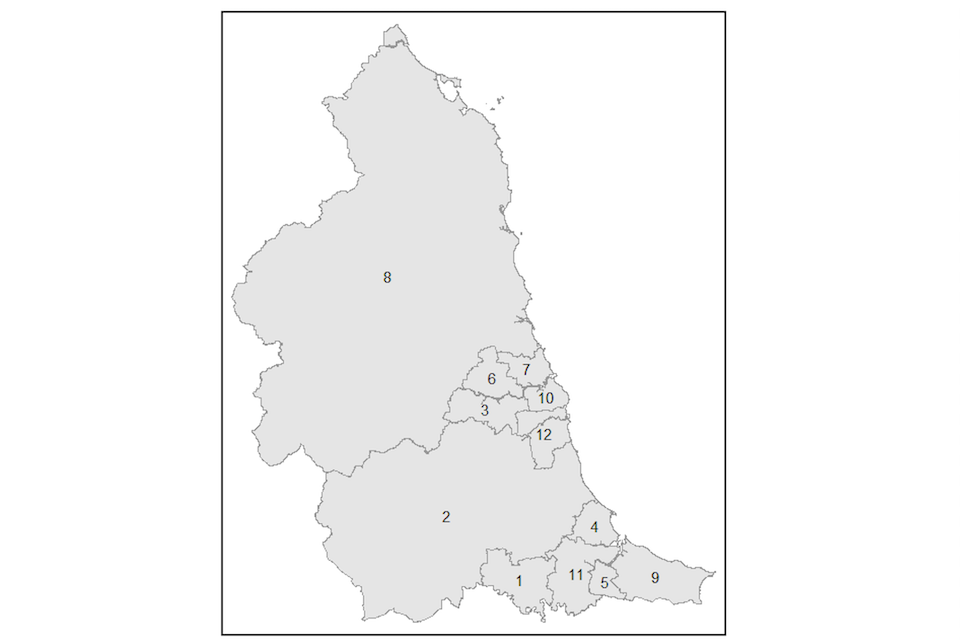
Figure 4.2: Local authorities in the North West of England

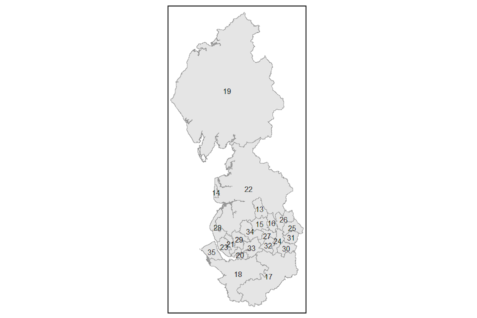
Figure 4.3: Local authorities in Yorkshire and the Humber

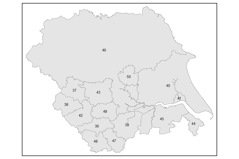
Figure 4.4: Local authorities in the East Midlands

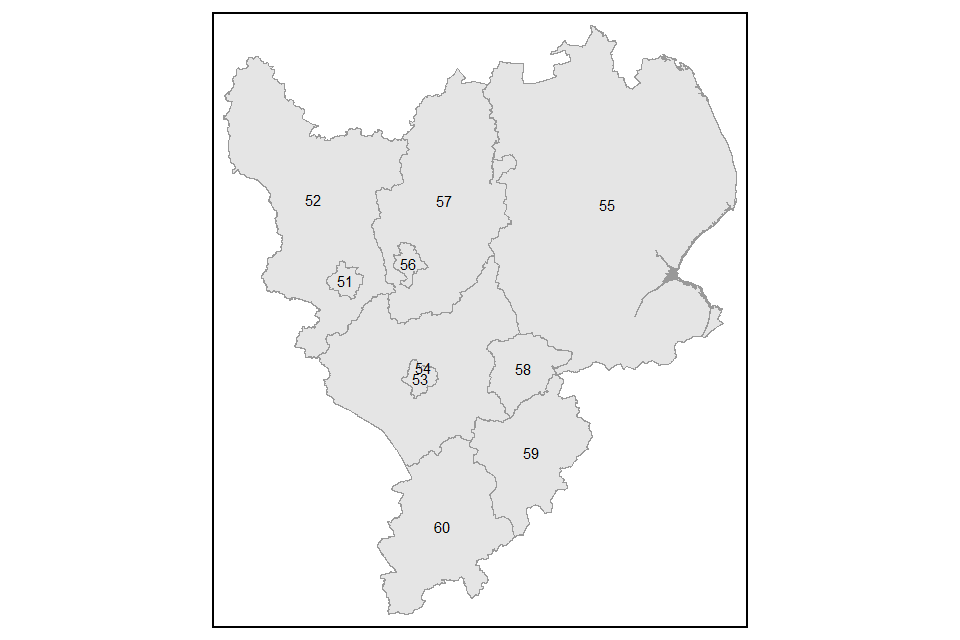
Figure 4.5: Local authorities in the West Midlands

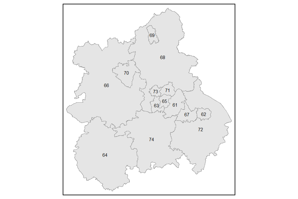
Figure 4.6: Local authorities in the East of England

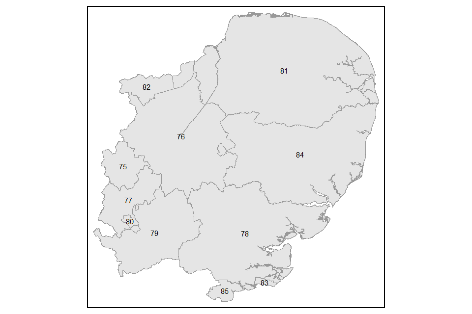
Figure 4.7: Local authorities in London

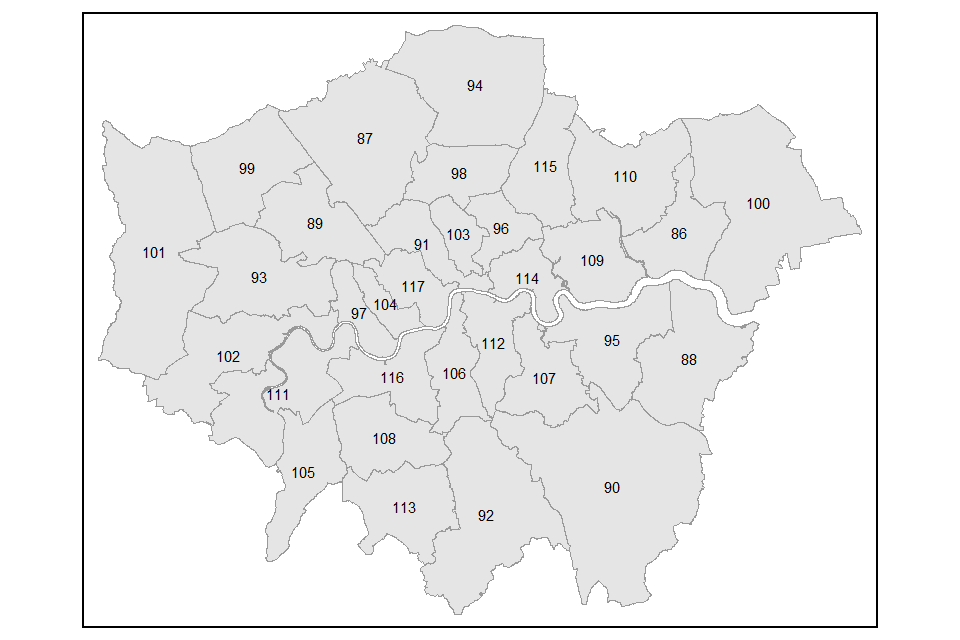
Figure 4.8: Local authorities in the South East of England

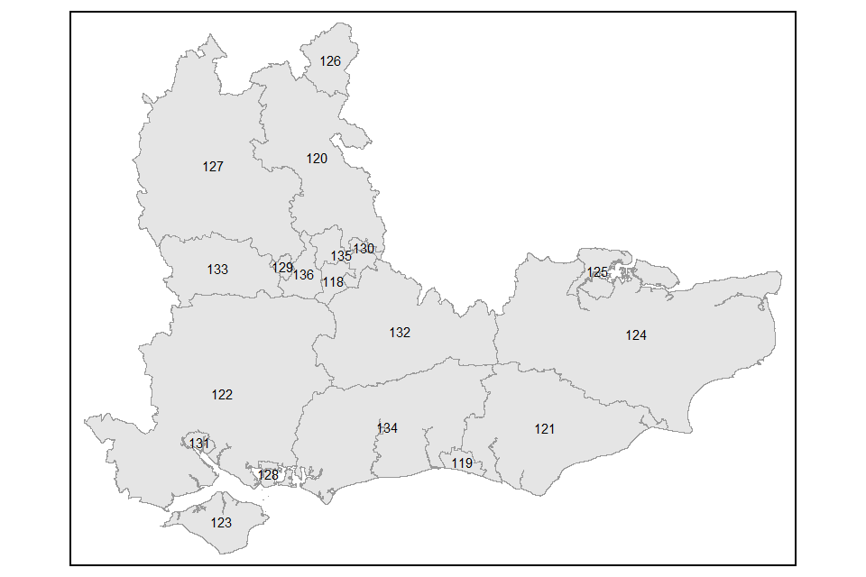
Figure 4.9: Local authorities in the South West of England

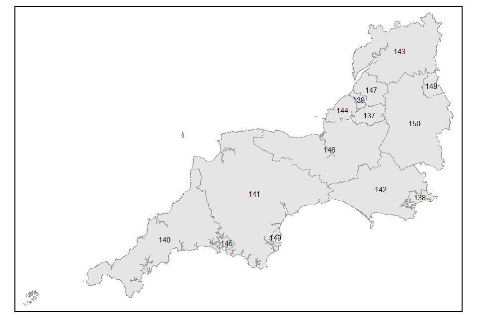
Figure 4.10: Local authorities in Scotland

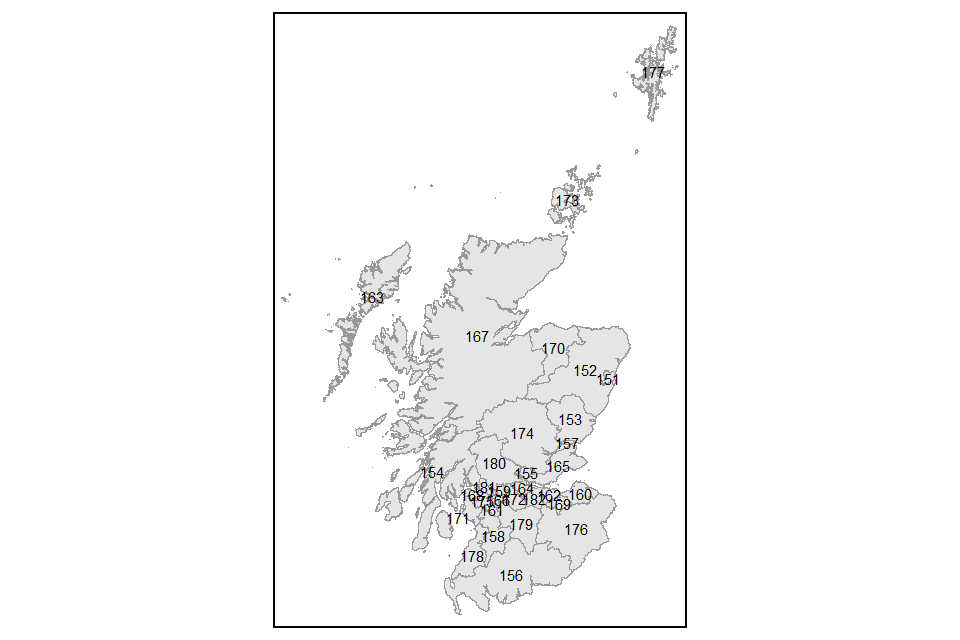
Figure 4.11: Local authorities in Wales

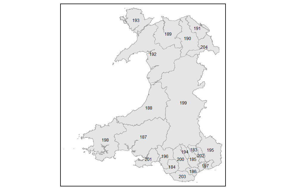
Figure 4.12: Local authorities in Northern Ireland

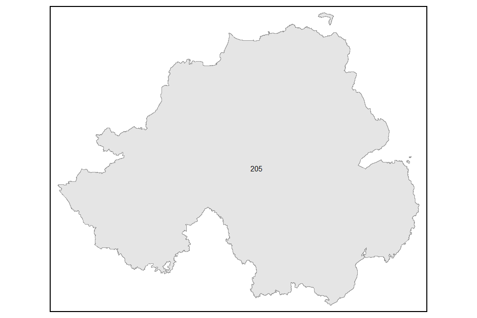
4.3 List of Travel to Work Areas (TTWAs)

Table 4.3: The 228 TTWAs in the UK

Travel to work area name	Number
Berwick	1
Blyth and Ashington	2
Carlisle	3
Darlington	4
Durham and Bishop Auckland	5
Hartlepool	6
Hawick and Kelso	7
Hexham	8
Middlesbrough and Stockton	9
Newcastle	10
Northallerton	11
Penrith	12
Sunderland	13
Whitby	14
Barrow-in-Furness	15
Birkenhead	16
Blackburn	17
Blackpool	18
Bradford	19
Burnley	20
Buxton	21
Chester	22
Crewe	23
Halifax	24
Huddersfield	25
Kendal	26
Lancaster and Morecambe	27
Liverpool	28
Manchester	29
Preston	30
Shrewsbury	31
Skipton	32
Stoke-on-Trent	33
Warrington and Wigan	34
Whitehaven	35
Workington	36
Wrexham	37
Barnsley	38
Bridlington	39
Chesterfield	40
Doncaster	41
Grimsby	42
Harrogate	43
Hull	44
Leeds	45
Lincoln	46
Malton	47
Scarborough	48
Scunthorpe	49
Sheffield	50
Wakefield and Castleford	51
Worksop and Retford	52
York	53
Banbury	54
Bedford	55
Birmingham	56
Boston	57
Burton upon Trent	58
Corby	59
Coventry	60
Derby	61
Grantham	62
Huntingdon	63
Kettering and Wellingborough	64
King’s Lynn	65
Leamington Spa	66
Leicester	67
Mansfield	68
Milton Keynes	69
Northampton	70
Nottingham	71
Oxford	72
Peterborough	73
Skegness and Louth	74
Spalding	75
Wisbech	76
Brecon	77
Cheltenham	78
Cinderford and Ross-on-Wye	79
Dudley	80
Evesham	81
Gloucester	82
Hereford	83
Llandrindod Wells and Builth Wells	84
Ludlow	85
Merthyr Tydfil	86
Newtown and Welshpool	87
Oswestry	88
Stafford	89
Telford	90
Wolverhampton and Walsall	91
Worcester and Kidderminster	92
Bury St Edmunds	93
Cambridge	94
Chelmsford	95
Clacton	96
Colchester	97
Cromer and Sheringham	98
Great Yarmouth	99
High Wycombe and Aylesbury	100
Ipswich	101
Lowestoft	102
Luton	103
Norwich	104
Southend	105
Stevenage and Welwyn Garden City	106
Thetford and Mildenhall	107
Crawley	108
Guildford and Aldershot	109
London	110
Slough and Heathrow	111
Tunbridge Wells	112
Andover	113
Ashford	114
Basingstoke	115
Bournemouth	116
Brighton	117
Canterbury	118
Chichester and Bognor Regis	119
Eastbourne	120
Folkestone and Dover	121
Hastings	122
Isle of Wight	123
Margate and Ramsgate	124
Medway	125
Newbury	126
Portsmouth	127
Reading	128
Salisbury	129
Southampton	130
Swindon	131
Worthing	132
Barnstaple	133
Bath	134
Bideford	135
Blandford Forum and Gillingham	136
Bridgwater	137
Bridport	138
Bristol	139
Bude	140
Dorchester and Weymouth	141
Exeter	142
Falmouth	143
Kingsbridge and Dartmouth	144
Launceston	145
Liskeard	146
Minehead	147
Newport	148
Penzance	149
Plymouth	150
Poole	151
Redruth and Truro	152
Sidmouth	153
St Austell and Newquay	154
Street and Wells	155
Taunton	156
Torquay and Paignton	157
Trowbridge	158
Wadebridge	159
Weston-super-Mare	160
Yeovil	161
Aberdeen	162
Alness and Invergordon	163
Arbroath and Montrose	164
Aviemore and Grantown-on-Spey	165
Ayr	166
Broadford and Kyle of Lochalsh	167
Campbeltown	168
Dalbeattie and Castle Douglas	169
Dumbarton and Helensburgh	170
Dumfries	171
Dundee	172
Dunfermline and Kirkcaldy	173
Dunoon and Rothesay	174
Edinburgh	175
Elgin	176
Falkirk and Stirling	177
Fort William	178
Fraserburgh	179
Galashiels and Peebles	180
Girvan	181
Glasgow	182
Golspie and Brora	183
Greenock	184
Inverness	185
Kilmarnock and Irvine	186
Livingston	187
Lochgilphead	188
Motherwell and Airdrie	189
Mull and Islay	190
Newton Stewart	191
Oban	192
Orkney Islands	193
Perth	194
Peterhead	195
Pitlochry and Aberfeldy	196
Portree	197
Shetland Islands	198
St Andrews and Cupar	199
Stranraer	200
Thurso	201
Turriff and Banff	202
Ullapool	203
Western Isles	204
Wick	205
Aberystwyth	206
Bangor and Holyhead	207
Bridgend	208
Cardiff	209
Cardigan	210
Colwyn Bay	211
Haverfordwest and Milford Haven	212
Llanelli	213
Pembroke and Tenby	214
Pwllheli and Porthmadog	215
Rhyl	216
Swansea	217
Tywyn and Dolgellau	218
Ballymena	219
Belfast	220
Coleraine	221
Cookstown and Magherafelt	222
Craigavon	223
Derry	224
Dungannon	225
Enniskillen	226
Newry and Banbridge	227
Omagh and Strabane	228

4.4 Travel to Work Areas within regions in the UK

The following maps show the 228 Travel to Work Areas (TTWAs) used in the analysis. TTWAs cross administrative boundaries and do not align directly with standard regions. They have been best-fitted into the regional categories below.

For more details on how local authorities map to their corresponding Travel to Work Areas, see:  Areas in TTW - MapIt 

Figure 4.13: TTWAs in the North East of England

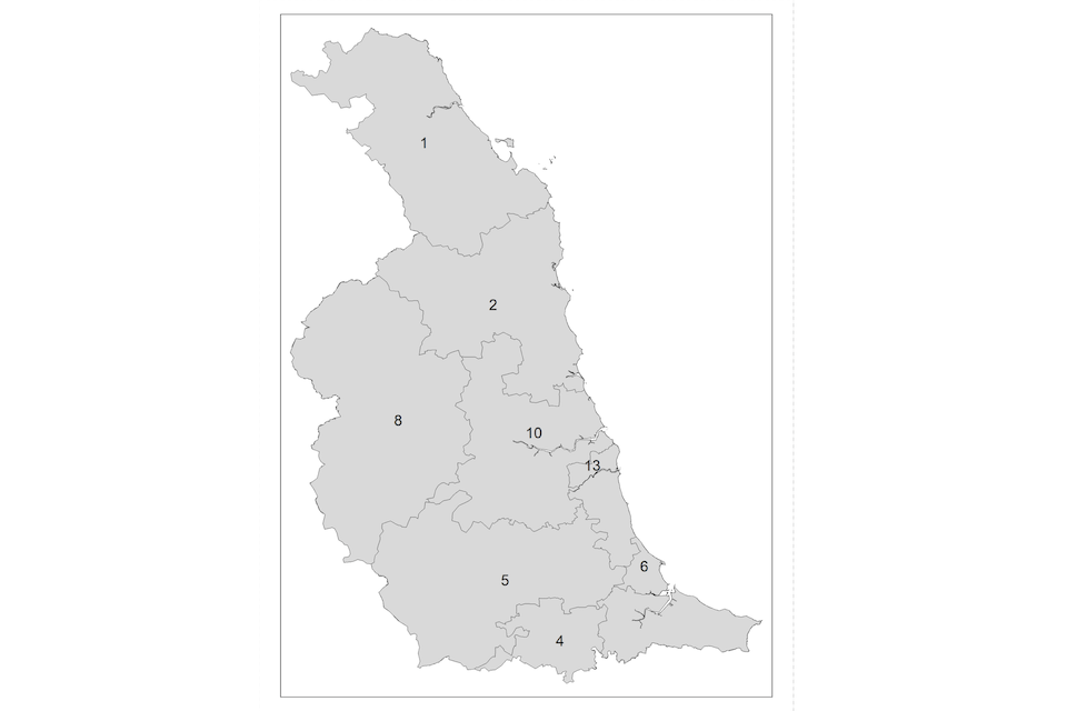
Figure 4.14: TTWAs in the North West of England

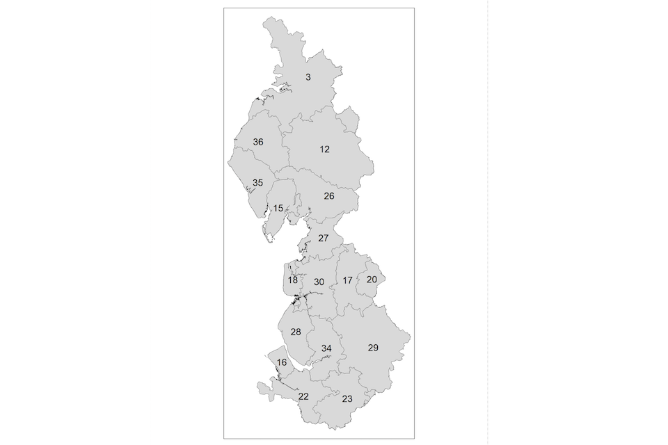
Figure 4.15: TTWAs in Yorkshire and the Humber

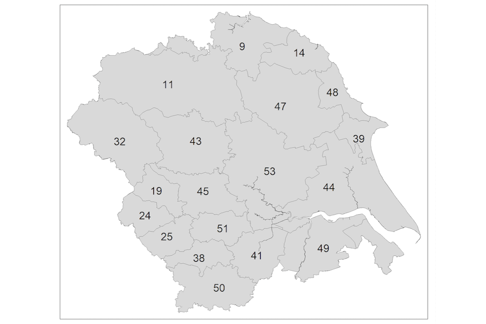
Figure 4.16: TTWAs in the East Midlands

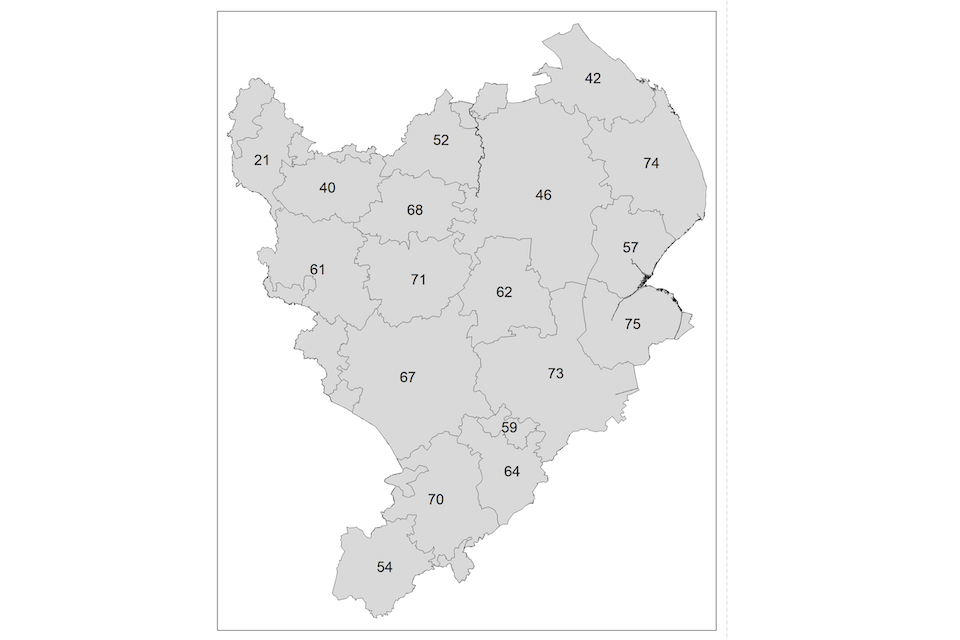
Figure 4.17: TTWAs in the West Midlands

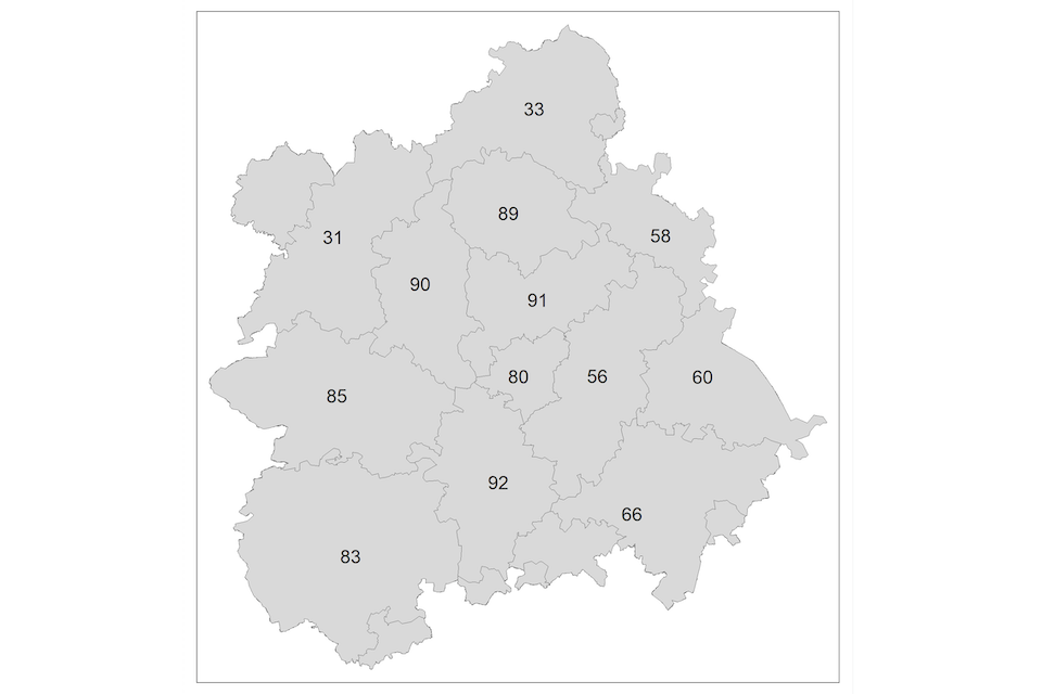
Figure 4.18: TTWAs in the East of England

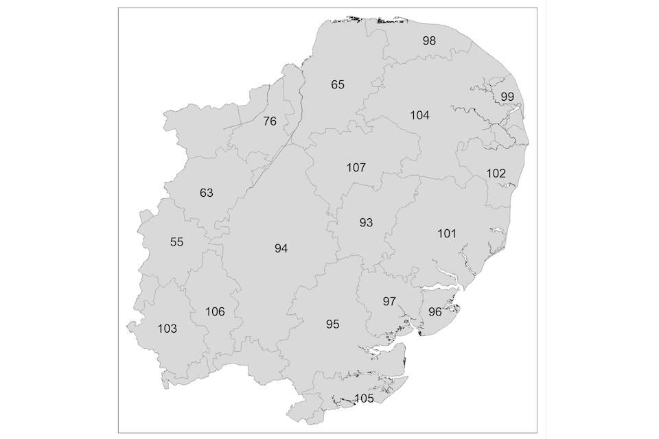
Figure 4.19: TTWAs in London and the South East

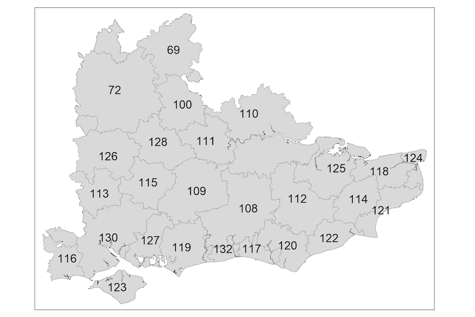
Figure 4.20: TTWAs in the South West of England

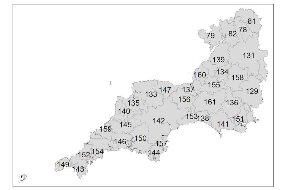
Figure 4.21: TTWAs in Scotland

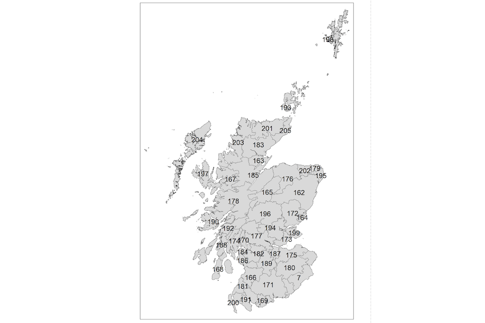
Figure 4.22: TTWAs in Wales

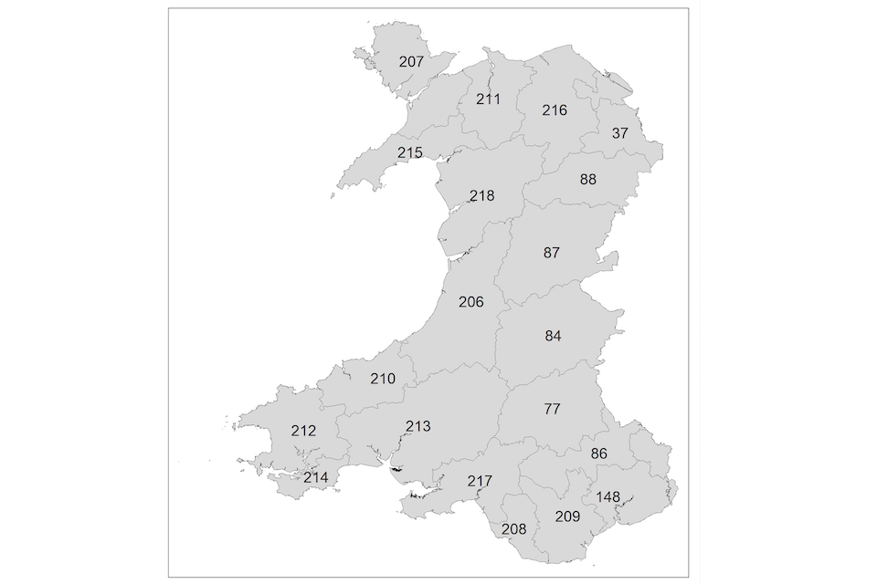
Figure 4.23: TTWAs in Northern Ireland

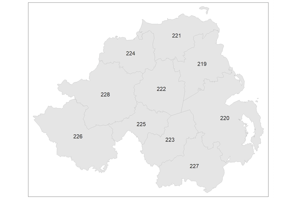
5. Limitations of the data and analysis

We have included a list of limitations with our analysis below. Please note, this list is non-exhaustive. Some of these limitations have previously been referenced in our 2024 and 2025 State of the Nation reports.

5.1 Lack of harmonised educational data from administrative sources across the UK

Historically, Scotland has had its own educational system and qualifications separate from the rest of the UK. Since devolution, state education has become a separate responsibility of each of the 4 nations: the Department for Education in England, the Scottish Government through its executive agency, Education Scotland, the Department for Education and Skills in Wales and the Department of Education in Northern Ireland. As a result, there are separate statistical series for each of the 4 nations’ administrative data on state education, reflecting local needs, with no UK-wide harmonised data.

5.2 Lack of coverage of the full population in the datasets

There are likely to be problems of under-coverage and of response bias both in the sample surveys and in administrative data used in the Social Mobility Index. For example, sample surveys such as the LFS sample private households but exclude residents of communal establishments (such as care homes). Similarly administrative data from the DfE covers children at maintained schools but may exclude those in private schools or children who are home-schooled. In addition, even among children who should be covered by the data in principle, there will be issues of non-response bias. So ‘hard to reach’ groups (such as undocumented residents) will tend to be under-represented in both administrative datasets and in sample surveys of the population. In the case of sample surveys, all of our data sources use weighting techniques in order to mitigate known biases (although weighting does not necessarily correct for all sources of potential bias). Weighting is not, however, used in the case of administrative data.

The LS and Census analysis have extremely high coverage. Because census agencies use statistical modelling to adjust for anyone missing from the survey, the final published datasets represent 100% of the estimated usual resident population. The ONS Census 2021 general report cites the final household response rate of England and Wales as 97%. The ONS longitudinal study samples approximately 1% of the Census for England and Wales at each Census. Since its inception in 1971 the study has captured individual level data for over 1.3 million sample members.

5.3 Limitations of the variables available in the dataset

The measures in the Social Mobility Index are not an exhaustive set of the potential drivers and outcomes of mobility. When selecting drivers and indicators for inclusion in the index, the main criterion has been whether quantitative data of sufficient quality is available over time for monitoring purposes, and whether there is sufficiently convincing evidence that the concept being measured is likely to have a causal (direct or indirect) influence on aggregate levels of social mobility. However, data on many factors that may be relevant for social mobility, such as social ties and social capital, is not often updated on a regular basis. Moreover, in some cases we have had to rely on proxy measures rather than direct measures of the concept in question (for example, eligibility for free school meals as a proxy for socio-economic background). As research in this area develops and the evidence base improves, we expect that the measures included in the Social Mobility Index will change over time.

5.4 Small sample sizes and imprecision of estimates

While our main administrative and survey data sources have a large number of respondents, the number of respondents in particular categories (for example certain ethnic groups) can occasionally be quite small. Consequently, this can lead to imprecision in the estimates as a result of sampling error (for more information, please see section 2.2 of this document). This is particularly likely to occur in intersectional analysis of geographical data, due to the small sample sizes that occur in small geographical regions. Small sample sizes can also increase the risk that individual respondents can be identified. For this reason the ONS does not release estimates when there are concerns about imprecision and disclosure. Furthermore, small sample sizes also limit the granularity of the data that can be analysed. Such as in the case of ethnic groups where highly simplified and heterogeneous categories have sometimes been used.

In some cases, we have had to report proportions that are estimated from a model, instead of the actual proportions we observed in the data. This is because the sample size in some subcategories is so low that the actual proportions may not be a very reliable indicator. In these cases, we have had to make simplifying assumptions, for example that the socio-economic background effect is similar across all ethnicities.

5.5 Measurement error

In addition to sampling error, our data is also likely affected by other forms of measurement error. If this error is randomly distributed, it will tend to weaken the strength of the measured associations between variables (so for example leading us to underestimate the strength of the association between socio-economic background and mobility outcomes).

However, not all measurement error is likely to be random and some types of non-random measurement error may lead to biases in the results. Problems of this kind are likely to be present with data that requires the respondent to recall information from when they were younger, such as their socio-economic background or the geographical area in which they grew up.

This is particularly true for questions of these types, which ask the respondent to recall socio-economic background or geographical region at the age of 14 specifically. Respondents whose families moved between areas, or whose parents changed jobs while they were growing up, may recall the most salient one from their youth rather than the one at age 14. A further complication with respect to historic geographical data is that local government regions have been reorganised, and hence respondents’ memories may not correspond with current administrative areas.

5.6 Limitations of descriptive analysis

Descriptive monitoring data on its own cannot tell us why a problem has emerged or what interventions would be successful in mitigating the problem. The primary function of the Social Mobility Index is to identify where more in-depth analyses are required in order to determine any underlying causal relationships, and to develop relevant social mobility policy accordingly.

5.7 Statistical analysis

The State of the Nation report and the Data Explorer Tool mainly rely on relatively simple statistical techniques such as bivariate cross-tabulations. These have the advantage of “staying close” to the data. In some cases, however, we have used modelling techniques in order to obtain reasonably precise estimates for groups with small sample sizes, such as ethnic minorities or geographical areas. These techniques (such as regression and multilevel modelling) borrow strength from the overall pattern of results in order to make estimates for the small group in question. However, they invariably require assumptions which cannot always be rigorously verified, due to, as an example, a lack of statistical power. The results derived from these modelling techniques should therefore be treated with caution.

5.8 Limitations of quantitative analysis

The measurement framework is designed to enable the SMC to fulfil its statutory duty of monitoring social mobility across the UK, and therefore utilises quantitative data. However, in order to fully understand the processes at work, particularly for the most disadvantaged areas or groups, other types of data such as cultural, social and institutional contexts may be needed. Ethnographic work can therefore be a valuable complement to statistical analysis.

6. Glossary

6.1 Absolute social mobility

This is the idea that some people have different life outcomes from their parents.

Absolute mobility rates look at the proportion of the population who are in different positions (often occupational class or income) from their parents, and are usually given as a simple percentage.

For example, a person experiences upward absolute income mobility if their income is greater than their parents’ income. They experience upward absolute occupational mobility if their occupation class is higher than their parents’. Mobility can also be downward.

6.2 Apprenticeships

A work-based training system, where apprentices earn a qualification after completing a blended mix of study and work.

Apprentices must complete 20% of their training off the job, be paid the apprenticeship minimum wage, and pass an end point assessment.

6.3 Caterpillar plots

A chart which shows both an estimate of a data point and a confidence interval (see definition in this glossary), arranged according to the magnitude of the estimates. The confidence interval usually is represented by a line going through the point which itself represents the estimated value in the chart.

6.4 Class pay gap

The difference in average pay between people who occupy the same type of job but come from different class backgrounds.

6.5 Composite index

An index consisting of multiple indicators. In our report they all consist of 3 different indicators. For example, our composite index on Promising Prospects consists of indicators on the highest level of qualification achieved, occupational class, and hourly earnings.

6.6 Conditional probability

Conditional probability is the chance that one event will occur based on the fact that another event has already taken place.

6.7 Confidence intervals

A range of values for which there is a defined probability (usually 95%) that an estimate lies within this range. For example if we have a confidence interval of 5 to 10 at the 95% level, we are 95% confident that our estimate lies within the range of values from 5 to 10.

6.8 Drivers

These capture the background conditions that make social mobility easier. For example, the availability of good education is a driver, because it helps people to be upwardly mobile. So our measures of drivers tell us about these nationwide background conditions. They do not tell us what the UK’s rates of mobility have been, and they are not broken down by socio-economic background.

6.9 Early years foundation stage profile (EYFSP)

The early years foundation stage profile (EYFSP) sets standards in England for the learning, development and care of a child from birth to 5 years old. All schools and Ofsted-registered early years providers must follow the EYFSP, including childminders, pre-schools, nurseries and school reception classes. There are different early years standards in Scotland, Wales and Northern Ireland.

6.10 Economically inactive

Individuals that are out of work and not looking for a job. Reasons for this include sickness, looking after family, and being a student, among others.

6.11 Free school meals (FSM)

In England, a free school meal (FSM) is a statutory benefit available to school-aged children from families who receive other qualifying benefits and who have been through the relevant registration process. FSM eligibility is often used as a proxy measure for disadvantage in school-aged children.

Free school meal eligibility is the only available measure of pupils’ social background in England, Wales and Northern Ireland. In Scotland, a completely different area-based measure of social background is used, the Scottish Index of Multiple Deprivation (SIMD).

FSM only includes those who have both applied for and been deemed eligible by the relevant local authority. It excludes an unknown number of people who might have been deemed eligible had they applied, and may also include some relatively affluent families.

6.12 Further education (FE)

Typically refers to classroom-based learning at further education (FE) colleges or providers. Students can start at age 14 or 16 years, depending on the college.

6.13 General Certificate of Secondary Education (GCSE)

The GCSE is an academic qualification taken in England, Wales and Northern Ireland, normally at age 16. State schools in Scotland use the Scottish Qualifications Certificate instead.

6.14 Higher education (HE)

Typically refers to post-secondary education, or tertiary education, leading to award of an academic degree. Higher education is an optional final stage of formal learning that occurs after completion of secondary education.

6.15 Income mobility

See social mobility, absolute social mobility and relative social mobility.

6.16 Intermediate (occupations)

See NS-SEC.

6.17 Intermediate outcomes

These capture the progress that people make from their starting point to an intermediate point, such as employment in their 20s, or educational attainment at 16. We break outcome measures down by people’s socio-economic background, so that we can see how different starting points affect progress to eventual end points.

6.18 International Territorial Level (ITL)

This is the internationally comparable regional geography for the UK. The regions that we use are part of a system developed by the Office for National Statistics (ONS). The level of the system we use, ITL2, divides the UK into 41 regions. Each region has between 800,000 and 3,000,000 inhabitants and contains about 4 upper-tier local authorities.

6.19 Key stage 2 (KS2)

The 4 years of schooling in England and Wales, described as year 3, year 4, year 5 and year 6, when pupils are aged between 7 and 11 years. Key stage 2 SATs (National Curriculum tests) are taken by pupils aged 11 years at the end of year 6, which is, usually, the final year in primary school.

6.20 Key stage 4 (KS4)

The 2 years from year 10 to year 11, when pupils are aged between 14 and 16 years. Most pupils take their final general certificate of secondary education (GCSE) exams at the end of year 11.

6.21 Labour Force Survey (LFS)

The LFS is a large-scale nationally-representative government survey that covers England, Wales, Scotland and Northern Ireland. The survey is managed by the Office for National Statistics (ONS) in Great Britain, and the Northern Ireland Statistics and Research Agency (NISRA) in Northern Ireland.

Its purpose is to provide information on the UK labour market which can then be used to develop, manage, evaluate and report on labour market policies.

6.22 Longitudinal study

The ONS Longitudinal Study (ONS-LS) contains linked census and life events data for a 1% sample of the population of England and Wales. It contains records on over 500,000 people usually resident in England and Wales at each point in time and is largely representative of the whole population.  The LS is the largest longitudinal data resource in England and Wales.

More information: Longitudinal Study 1971 to 1991 History, organisation and quality of data.

6.23 Mobility outcomes

These capture the progress people have made compared to their parents at a later point in life (often in one’s 50s).

6.24 Moving average model

A moving average is a method of smoothing data by calculating the average of a set number of recent data points.

6.25 Multilevel model

This is a statistical model which takes account of the clustering of individuals within higher-level units such as regions or schools.

6.26 National Minimum Wage

The minimum wage that an employer must pay its workforce. As of April 2026, the minimum wage is set at £12.71 for those aged over 21 years old. This is also known as the “national living wage”. There are lower national minimum wage amounts for younger people. In this report, this is referred to as the minimum wage.

6.27 National Statistics Socio-economic Classification (NS-SEC)

This is the best national measure to monitor occupational social mobility. We define an individual’s socio-economic background according to the occupation of their higher- earning parent. This year we use a 5 part grouping:

• Higher professional: NS-SEC 1. Examples of which include CEOs, doctors and engineers.
• Lower professional: NS-SEC 2. Examples of which include teachers, nurses and journalists
• Intermediate: NS-SEC 3 and 4. Examples of which include shopkeepers, taxi drivers and roofers.
• Higher working class: NS-SEC 5 and 6. Examples of which include mechanics, electricians and housekeepers.
• Lower working class: NS-SEC 7 and 8. Examples of which include cleaners, porters and waiters.

6.28 Not in education, employment or training (NEET)

The annual publication of national participation figures of young people aged 16 to 18 years includes a measure of those who are NEET (not in education, employment or training).

6.29 Occupational mobility

See social mobility, absolute social mobility and relative social mobility

6.30 Occupational wage

Occupational wages are the average wage for each occupation. They are estimated indirectly from other data sources. In our analysis the occupational wage was imputed into the ONS-LS using earnings data from the ASHE.

6.31 Odds ratio

The odds ratio is a statistic which can be used for comparing the mobility chances of people from different socio-economic backgrounds. It can be thought of as a way of assessing the outcome of a competition between people from 2 different backgrounds to achieve an advantaged outcome and to avoid a disadvantaged outcome.

A log odds ratio is the natural logarithm of an odds ratio. It transforms a skewed ratio measuring the association between two events into a symmetrical value centred at zero, making it useful for statistical modelling like logistic regression.

6.32 Organisation for Economic Co-operation and Development (OECD)

The OECD is an international organisation of 38 countries committed to democracy and the market economy. We use the 37 other member states as international comparators to the UK.

6.33 Pay As You Earn (PAYE)

Most people pay Income Tax through PAYE. This is the system the employer or pension provider uses to take Income Tax and National Insurance contributions before they pay wages or pension. Your tax code tells your employer how much to deduct.

6.34 Professional, professional/ managerial (occupations)

See NS-SEC.

6.35 Programme for International Student Assessment (PISA)

PISA is the OECD’s Programme for International Student Assessment. PISA measures 15-year-olds’ ability to use their reading, mathematics and science knowledge and skills to meet real-life challenges.

6.36 Pupil Premium

A sum of money given by the UK government to schools in England to improve the attainment of disadvantaged children.

6.37 Quintile

20% of a population which is usually ordered in either ascending or descending order of some metric. After being ranked, the population is split into 5 equal sized groups, and each of these groups is one quintile.

6.38 Random effects model

A type of statistical model in which one or more of the model parameters is a random variable.

6.39 Relative poverty

This is one measure of poverty. A household is in relative poverty if its income is below 60% of the average (median) net household income in the same year. In other words, the pound amount of the poverty line changes each year based on current median income in the country.

6.40 Relative social mobility

Relative mobility involves a comparison of the positions of people from different social backgrounds. For example, in the case of income, relative mobility tells us how strongly children’s ranking within their income distribution is associated with their parents’ ranking. Relative mobility is low if almost everyone ends up with a similar rank as their parents. For example, if parents in the bottom decile of earnings have children that mostly end up in the bottom decile of earnings.

While absolute and relative social mobility often go together, they are not the same concept. For example, if a society creates more professional jobs, absolute occupational mobility should improve. But if most of these professional jobs go to people from professional backgrounds, relative social mobility may remain static.

6.41 Social mobility

Social mobility refers to movement within a given stratification system. Social mobility can be either intergenerational (when children move away from their parents’ position) or intra-generational (when people move away from their own initial position). There are different dimensions of stratification – we focus on the key mobility dimension of occupational class, and add further dimensions like income, wealth, education and housing, as the data allows. See also the distinction between relative social mobility and absolute social mobility.

6.42 Social Mobility Index (SMI)

The Social Mobility Index is a long-term measurement framework for social mobility in the UK. It replaces the Commission’s original Social Mobility Index, launched in 2016. This new Index provides a critical starting point to improve the evidence base and goes well beyond solely reporting on the drivers of mobility.

We report on social mobility outcomes which show where people end up in comparison with where they started. This is across a range of outcomes of interest, including occupational class, income, education, and either at an earlier stage in their lives in their 20s and 30s (intermediate outcomes), or a later stage in their 40s and 50s (mobility outcomes).

6.43 Socio-economic classification, background

See NS-SEC.

6.44 Travel to Work Area (TTWA)

Travel-to-Work Areas (TTWAs) are a non-administrative geographical classification framework developed by the ONS to reflect functional local labour markets. They are constructed using census commuting flow matrices to ensure a high degree of economic self-containment. For more information see section 3.3.

A geographic zone qualifies as a TTWA if it meets the standard ONS self-containment criteria based on the economically active population:

• a minimum of 75% of the area’s resident workforce must be locally employed within the same area
• a minimum of 75% of the jobs within the area must be filled by local residents

More information: ONS Travel to Work Areas Methodological Guidance.

6.45 Unidiff parameters

The Unidiff parameter provides a single number to show whether the level of relative mobility (as measured by log odds ratios) differs across the tables being compared. This allows us to compare levels of relative mobility across, for example, different years, or different ethnicities.

6.46 Universities and Colleges Admissions Service (UCAS)

The Universities and Colleges Admissions Service – a nonprofit organisation which conducts the application process for UK universities.

6.47 Understanding Society, The UK Household Longitudinal Survey (UKHLS)

The UKHLS is a longitudinal survey of the members of approximately 40,000 households in the UK. The study is based at the Institute for Social and Economic Research at the University of Essex.

The purpose of UKHLS is to provide high-quality longitudinal data on subjects such as health, work, education, income, family, and social life. This helps to understand the long-term effects of social and economic change, as well as policy interventions designed to impact the general wellbeing of the UK population.

6.48 Wealth and Assets Survey (WAS)

A longitudinal survey of around 17,000 households conducted by ONS every 2 years. The purpose of the survey is to ‘measure the well-being of households and individuals in terms of their assets, savings, debt and planning for retirement’.

6.49 Working-class occupations

See NS-SEC.

7. Supplementary tables of ONS-LS analysis

These tables show supplementary analysis using the ONS Longitudinal Study.

7.1 Educational mobility, early Career

Sample: All

Census: 1971 to 1991

Mobility table: Education, age 28-37, sample = All, census = 1971 to 1991

Parent	Children Degree level and higher	Children Sub-degree/none/unknown/ other	Total
One or both parent degree	1,243 (49.0%)	1,293 (51.0%)	2,536
Neither parent degree	5,373 (9.0%)	54,448 (91.0%)	59,821
Total	6,616	55,741	62,357

Source: ONS-Longitudinal Study

Sample: All

Census: 1981 to 2001

Mobility table: Education, age 28-37, sample = All, census = 1981 to 2001

Parent	Children Degree level and higher	Children Sub-degree/none/unknown/ other	Total
One or both parent degree	3,384 (64.4%)	1,872 (35.6%)	5,256
Neither parent degree	10,942 (19.0%)	46,783 (81.0%)	57,725
Total	14,326	48,655	62,981

Source: ONS-Longitudinal Study

Sample: All

Census: 1991 to 2011

Mobility table: Education, age 28-37, sample = All, census = 1991 to 2011

Parent	Children Degree level and higher	Children Sub-degree/none/unknown/ other	Total
One or both parent degree	4,503 (79.5%)	1,159 (20.5%)	5,662
Neither parent degree	15,506 (34.7%)	29,195 (65.3%)	44,701
Total	20,009	30,354	50,363

Source: ONS-Longitudinal Study

Sample: All

Census: 2001 to 2021

Mobility table: Education, age 28-37, sample = All, census = 2001 to 2021

Parent	Children Degree level and higher	Children Sub-degree/none/unknown/ other	Total
One or both parent degree	10,123 (70.5%)	4,244 (29.5%)	14,367
Neither parent degree	15,876 (37.8%)	26,160 (62.2%)	42,036
Total	25,999	30,404	56,403

Source: ONS-Longitudinal Study

Sample: Female

Census: 1971 to 1991

Mobility table: Education, age 28-37, sample = Female, census = 1971 to 1991

Parent	Daughters Degree level and higher	Daughters Sub-degree/none/unknown/ other	Total
One or both parent degree	561 (45.0%)	685 (55.0%)	1,246
Neither parent degree	2,186 (7.3%)	27,783 (92.7%)	29,969
Total	2,747	28,468	31,215

Source: ONS-Longitudinal Study

Sample: Female

Census: 1981 to 2001

Mobility table: Education, age 28-37, sample = Female, census = 1981 to 2001

Parent	Daughters Degree level and higher	Daughters Sub-degree/none/unknown/ other	Total
One or both parent degree	1,684 (63.5%)	969 (36.5%)	2,653
Neither parent degree	5,520 (18.5%)	24,313 (81.5%)	29,833
Total	7,204	25,282	32,486

Source: ONS-Longitudinal Study

Sample: Female

Census: 1991 to 2011

Mobility table: Education, age 28-37, sample = Female, census = 1991 to 2011

Parent	Daughters Degree level and higher	Daughters Sub-degree/none/unknown/ other	Total
One or both parent degree	2,296 (81.3%)	527 (18.7%)	2,823
Neither parent degree	8,573 (37.1%)	14,502 (62.9%)	23,075
Total	10,869	15,029	25,898

Source: ONS-Longitudinal Study

Sample: Female

Census: 2001 to 2021

Mobility table: Education, age 28-37, sample = Female, census = 2001 to 2021

Parent	Daughters Degree level and higher	Daughters Sub-degree/none/unknown/ other	Total
One or both parent degree	5,428 (74.6%)	1,848 (25.4%)	7,276
Neither parent degree	9,113 (42.1%)	12,550 (57.9%)	21,663
Total	14,541	14,398	28,939

Source: ONS-Longitudinal Study

Sample: Male

Census: 1971 to 1991

Mobility table: Education, age 28-37, sample = Male, census = 1971 to 1991

Parent	Sons Degree level and higher	Sons Sub-degree/none/unknown/ other	Total
One or both parent degree	682 (52.9%)	608 (47.1%)	1,290
Neither parent degree	3,187 (10.7%)	26,665 (89.3%)	29,852
Total	3,869	27,273	31,142

Source: ONS-Longitudinal Study

Sample: Male

Census: 1981 to 2001

Mobility table: Education, age 28-37, sample = Male, census = 1981 to 2001

Parent	Sons Degree level and higher	Sons Sub-degree/none/unknown/ other	Total
One or both parent degree	1,700 (65.3%)	903 (34.7%)	2,603
Neither parent degree	5,422 (19.4%)	22,470 (80.6%)	27,892
Total	7,122	23,373	30,495

Source: ONS-Longitudinal Study

Sample: Male

Census: 1991 to 2011

Mobility table: Education, age 28-37, sample = Male, census = 1991 to 2011

Parent	Sons Degree level and higher	Sons Sub-degree/none/unknown/ other	Total
One or both parent degree	2,207 (77.7%)	632 (22.3%)	2,839
Neither parent degree	6,933 (32.1%)	14,693 (67.9%)	21,626
Total	9,140	15,325	24,465

Source: ONS-Longitudinal Study

Sample: Male

Census: 2001 to 2021

Mobility table: Education, age 28-37, sample = Male, census = 2001 to 2021

Parent	Sons Degree level and higher	Sons Sub-degree/none/unknown/ other	Total
One or both parent degree	4,695 (66.2%)	2,396 (33.8%)	7,091
Neither parent degree	6,763 (33.2%)	13,610 (66.8%)	20,373
Total	11,458	16,006	27,464

Source: ONS-Longitudinal Study

7.2 Housing mobility, early career

Sample: All

Census: 1971 to 1991

Mobility table: Housing, age 28-37, sample = All, census = 1971 to 1991

Parent	Children Owner	Children Renter	Total
Owner	26,234 (84.9%)	4,655 (15.1%)	30,889
Renter	21,524 (66.3%)	10,923 (33.7%)	32,447
Total	47,758	15,578	63,336

Source: ONS-Longitudinal Study

Sample: All

Census: 1981 to 2001

Mobility table: Housing, age 28-37, sample = All, census = 1981 to 2001

Parent	Children Owner	Children Renter	Total
Owner	33,636 (82.9%)	6,941 (17.1%)	40,577
Renter	14,311 (61.0%)	9,155 (39.0%)	23,466
Total	47,947	16,096	64,043

Source: ONS-Longitudinal Study

Sample: All

Census: 1991 to 2011

Mobility table: Housing, age 28-37, sample = All, census = 1991 to 2011

Parent	Children Owner	Children Renter	Total
Owner	28,121 (73.6%)	10,096 (26.4%)	38,217
Renter	5,391 (42.9%)	7,185 (57.1%)	12,576
Total	33,512	17,281	50,793

Source: ONS-Longitudinal Study

Sample: All

Census: 2001 to 2021

Mobility table: Housing, age 28-37, sample = All, census = 2001 to 2021

Parent	Children Owner	Children Renter	Total
Owner	29,662 (71.3%)	11,918 (28.7%)	41,580
Renter	5,490 (34.9%)	10,240 (65.1%)	15,730
Total	35,152	22,158	57,310

Source: ONS-Longitudinal Study

Sample: Female

Census: 1971 to 1991

Mobility table: Housing, age 28-37, sample = Female, census = 1971 to 1991

Parent	Daughters Owner	Daughters Renter	Total
Owner	12,845 (84.0%)	2,456 (16.1%)	15,301
Renter	10,799 (65.3%)	5,741 (34.7%)	16,540
Total	23,644	8,197	31,841

Source: ONS-Longitudinal Study

Sample: Female

Census: 1981 to 2001

Mobility table: Housing, age 28-37, sample = Female, census = 1981 to 2001

Parent	Daughters Owner	Daughters Renter	Total
Owner	16,947 (81.8%)	3,759 (18.1%)	20,706
Renter	7,271 (58.1%)	5,237 (41.9%)	12,508
Total	24,218	8,996	33,214

Source: ONS-Longitudinal Study

Sample: Female

Census: 1991 to 2011

Mobility table: Housing, age 28-37, sample = Female, census = 1991 to 2011

Parent	Daughters Owner	Daughters Renter	Total
Owner	14,157 (72.7%)	5,309 (27.3%)	19,466
Renter	2,756 (40.5%)	4,057 (59.5%)	6,813
Total	16,913	9,366	26,279

Source: ONS-Longitudinal Study

Sample: Female

Census: 2001 to 2021

Mobility table: Housing, age 28-37, sample = Female, census = 2001 to 2021

Parent	Daughters Owner	Daughters Renter	Total
Owner	14,677 (69.3%)	6,500 (30.7%)	21,177
Renter	2,731 (32.6%)	5,635 (67.4%)	8,366
Total	17,408	12,135	29,543

Source: ONS-Longitudinal Study

Sample: Male

Census: 1971 to 1991

Mobility table: Housing, age 28-37, sample = Male, census = 1971 to 1991

Parent	Sons Owner	Sons Renter	Total
	Owner	Renter	Total
Owner	13,389 (85.9%)	2,199 (14.1%)	15,588
Renter	10,725 (67.4%)	5,182 (32.6%)	15,907
Total	24,114	7,381	31,495

Source: ONS-Longitudinal Study

Sample: Male

Census: 1981 to 2001

Mobility table: Housing, age 28-37, sample = Male, census = 1981 to 2001

Parent	Sons Owner	Sons Renter	Total
Owner	16,689 (84.0%)	3,182 (16.0%)	19,871
Renter	7,040 (64.2%)	3,918 (35.8%)	10,958
Total	23,729	7,100	30,829

Source: ONS-Longitudinal Study

Sample: Male

Census: 1991 to 2011

Mobility table: Housing, age 28-37, sample = Male, census = 1991 to 2011

Parent	Sons Owner	Sons Renter	Total
Owner	13,964 (74.5%)	4,787 (25.5%)	18,751
Renter	2,635 (45.7%)	3,128 (54.3%)	5,763
Total	16,599	7,915	24,514

Source: ONS-Longitudinal Study

Sample: Male

Census: 2001 to 2021

Mobility table: Housing, age 28-37, sample = Male, census = 2001 to 2021

Parent	Sons Owner	Sons Renter	Total
Owner	14,985 (73.5%)	5,418 (26.6%)	20,403
Renter	2,759 (37.5%)	4,605 (62.5%)	7,364
Total	17,744	10,023	27,767

Source: ONS-Longitudinal Study

7.3 Housing mobility, mid career

Sample: All

Census: 1971 to 2001

Mobility table: Housing, age 38-47, sample = All, census = 1971 to 2001

Parent	Children Owner	Children Renter	Total
Owner	26,398 (88.1%)	3,555 (11.9%)	29,953
Renter	22,913 (74.0%)	8,031 (25.9%)	30,944
Total	49,311	11,586	60,897

Source: ONS-Longitudinal Study

Sample: All

Census: 1981 to 2011

Mobility table: Housing, age 38-47, sample = All, census = 1981 to 2011

Parent	Children Owner	Children Renter	Total
Owner	33,854 (83.3%)	6,775 (16.7%)	40,629
Renter	14,776 (62.4%)	8,912 (37.6%)	23,688
Total	48,630	15,687	64,317

Source: ONS-Longitudinal Study

Sample: All

Census: 1991 to 2021

Mobility table: Housing, age 38-47, sample = All, census = 1991 to 2021

Parent	Children Owner	Children Renter	Total
Owner	30,998 (78.4%)	8,543 (21.6%)	39,541
Renter	6,288 (47.0%)	7,090 (53.0%)	13,378
Total	37,286	15,633	52,919

Source: ONS-Longitudinal Study

Sample: Female

Census: 1971 to 2001

Mobility table: Housing, age 38-47, sample = Female, census = 1971 to 2001

Parent	Daughters Owner	Daughters Renter	Total
Owner	13,153 (87.5%)	1,875 (12.5%)	15,028
Renter	11,574 (72.7%)	4,341 (27.3%)	15,915
Total	24,727	6,216	30,943

Source: ONS-Longitudinal Study

Sample: Female

Census: 1981 to 2011

Mobility table: Housing, age 38-47, sample = Female, census = 1981 to 2011

Parent	Daughters Owner	Daughters Renter	Total
Owner	17,221 (83.1%)	3,508 (16.9%)	20,729
Renter	7,559 (60.7%)	4,899 (39.3%)	12,458
Total	24,780	8,407	33,187

Source: ONS-Longitudinal Study

Sample: Female

Census: 1991 to 2021

Mobility table: Housing, age 38-47, sample = Female, census = 1991 to 2021

Parent	Daughters Owner	Daughters Renter	Total
Owner	15,533 (77.4%)	4,539 (22.6%)	20,072
Renter	3,186 (44.8%)	3,929 (55.2%)	7,115
Total	18,719	8,468	27,187

Source: ONS-Longitudinal Study

Sample: Male

Census: 1971 to 2001

Mobility table: Housing, age 38-47, sample = Male, census = 1971 to 2001

Parent	Sons Owner	Sons Renter	Total
Owner	13,245 (88.7%)	1,680 (11.3%)	14,925
Renter	11,339 (75.5%)	3,690 (24.6%)	15,029
Total	24,584	5,370	29,954

Source: ONS-Longitudinal Study

Sample: Male

Census: 1981 to 2011

Mobility table: Housing, age 38-47, sample = Male, census = 1981 to 2011

Parent	Sons Owner	Sons Renter	Total
Owner	16,633 (83.6%)	3,267 (16.4%)	19,900
Renter	7,217 (64.3%)	4,013 (35.7%)	11,230
Total	23,850	7,280	31,130

Source: ONS-Longitudinal Study

Sample: Male

Census: 1991 to 2021

Mobility table: Housing, age 38-47, sample = Male, census = 1991 to 2021

Parent	Sons Owner	Sons Renter	Total
Owner	15,465 (79.4%)	4,004 (20.6%)	19,469
Renter	3,102 (49.5%)	3,161 (50.5%)	6,263
Total	18,567	7,165	25,732

Source: ONS-Longitudinal Study

7.4 Occupational mobility, early career, three classes

Sample: All

Census: 1971 to 1991

Mobility table: Occupational, age 28-37, sample = All, census = 1971 to 1991

Parent	Children Professional	Children Intermediate	Children Working	Total
Professional	6,795 (50.1%)	3,902 (28.8%)	2,866 (21.1%)	13,563
Intermediate	3,362 (33.3%)	3,295 (32.7%)	3,429 (34.0%)	10,086
Working	6,868 (22.4%)	8,343 (27.2%)	15,459 (50.4%)	30,670
Total	17,025	15,540	21,754	54,319

Source: ONS-Longitudinal Study

Sample: All

Census: 1981 to 2001

Mobility table: Occupational, age 28-37, sample = All, census = 1981 to 2001

Parent	Children Professional	Children Intermediate	Children Working	Total
Professional	10,063 (57.0%)	3,719 (21.1%)	3,887 (22.0%)	17,669
Intermediate	4,129 (40.7%)	2,589 (25.5%)	3,432 (33.8%)	10,150
Working	8,954 (31.3%)	6,000 (21.0%)	13,642 (47.7%)	28,596
Total	23,146	12,308	20,961	56,415

Source: ONS-Longitudinal Study

Sample: All

Census: 1991 to 2011

Mobility table: Occupational, age 28-37, sample = All, census = 1991 to 2011

Parent	Children Professional	Children Intermediate	Children Working	Total
Professional	9,445 (62.8%)	3,171 (21.1%)	2,429 (16.1%)	15,045
Intermediate	4,891 (45.0%)	3,040 (27.9%)	2,946 (27.1%)	10,877
Working	6,308 (35.2%)	4,538 (25.3%)	7,085 (39.5%)	17,931
Total	20,644	10,749	12,460	43,853

Source: ONS-Longitudinal Study

Sample: All

Census: 2001 to 2021

Mobility table: Occupational, age 28-37, sample = All, census = 2001 to 2021

Parent	Children Professional	Children Intermediate	Children Working	Total
Professional	11,825 (61.0%)	4,123 (21.3%)	3,427 (17.7%)	19,375
Intermediate	5,126 (47.5%)	3,019 (28.0%)	2,651 (24.6%)	10,796
Working	7,486 (37.1%)	5,001 (24.8%)	7,703 (38.1%)	20,190
Total	24,437	12,143	13,781	50,361

Source: ONS-Longitudinal Study

Sample: Female

Census: 1971 to 1991

Mobility table: Occupational, age 28-37, sample = Female, census = 1971 to 1991

Parent	Daughters Professional	Daughters Intermediate	Daughters Working	Total
Professional	2,841 (43.6%)	2,233 (34.3%)	1,440 (22.1%)	6,514
Intermediate	1,468 (30.2%)	1,770 (36.5%)	1,617 (33.3%)	4,855
Working	2,841 (19.8%)	4,606 (32.2%)	6,875 (48.0%)	14,322
Total	7,150	8,609	9,932	25,691

Source: ONS-Longitudinal Study

Sample: Female

Census: 1981 to 2001

Mobility table: Occupational, age 28-37, sample = Female, census = 1981 to 2001

Parent	Daughters Professional	Daughters Intermediate	Daughters Working	Total
Professional	4,722 (52.7%)	2,255 (25.2%)	1,977 (22.1%)	8,954
Intermediate	2,029 (39.3%)	1,401 (27.1%)	1,738 (33.6%)	5,168
Working	4,361 (29.7%)	3,643 (24.8%)	6,673 (45.5%)	14,677
Total	11,112	7,299	10,388	28,799

Source: ONS-Longitudinal Study

Sample: Female

Census: 1991 to 2011

Mobility table: Occupational, age 28-37, sample = Female, census = 1991 to 2011

Parent	Daughters Professional	Daughters Intermediate	Daughters Working	Total
Professional	4,723 (62.4%)	1,763 (23.3%)	1,083 (14.3%)	7,569
Intermediate	2,535 (46.4%)	1,589 (29.1%)	1,344 (24.6%)	5,468
Working	3,287 (35.9%)	2,655 (29.0%)	3,210 (35.1%)	9,152
Total	10,545	6,007	5,637	22,189

Source: ONS-Longitudinal Study

Sample: Female

Census: 2001 to 2021

Mobility table: Occupational, age 28-37, sample = Female, census = 2001 to 2021

Parent	Daughters Professional	Daughters Intermediate	Daughters Working	Total
Professional	6,016 (61.5%)	2,267 (23.2%)	1,506 (15.4%)	9,789
Intermediate	2,692 (49.6%)	1,513 (27.9%)	1,226 (22.6%)	5,431
Working	4,012 (38.5%)	2,732 (26.2%)	3,683 (35.3%)	10,427
Total	12,720	6,512	6,415	25,647

Source: ONS-Longitudinal Study

Sample: Male

Census: 1971 to 1991

Mobility table: Occupational, age 28-37, sample = Male, census = 1971 to 1991

Parent	Sons Professional	Sons Intermediate	Sons Working	Total
Professional	3,954 (56.1%)	1,669 (23.7%)	1,426 (20.2%)	7,049
Intermediate	1,894 (36.2%)	1,525 (29.1%)	1,812 (34.6%)	5,231
Working	4,027 (24.6%)	3,737 (22.9%)	8,584 (52.5%)	16,348
Total	9,875	6,931	11,822	28,628

Source: ONS-Longitudinal Study

Sample: Male

Census: 1981 to 2001

Mobility table: Occupational, age 28-37, sample = Male, census = 1981 to 2001

Parent	Sons Professional	Sons Intermediate	Sons Working	Total
Professional	5,341 (61.3%)	1,464 (16.8%)	1,910 (21.9%)	8,715
Intermediate	2,100 (42.1%)	1,188 (23.9%)	1,694 (34.0%)	4,982
Working	4,593 (33.0%)	2,357 (16.9%)	6,969 (50.1%)	13,919
Total	12,034	5,009	10,573	27,616

Source: ONS-Longitudinal Study

Sample: Male

Census: 1991 to 2011

Mobility table: Occupational, age 28-37, sample = Male, census = 1991 to 2011

Parent	Sons Professional	Sons Intermediate	Sons Working	Total
Professional	4,722 (63.2%)	1,408 (18.8%)	1,346 (18.0%)	7,476
Intermediate	2,356 (43.6%)	1,451 (26.8%)	1,602 (29.6%)	5,409
Working	3,021 (34.4%)	1,883 (21.4%)	3,875 (44.1%)	8,779
Total	10,099	4,742	6,823	21,664

Source: ONS-Longitudinal Study

Sample: Male

Census: 2001 to 2021

Mobility table: Occupational, age 28-37, sample = Male, census = 2001 to 2021

Parent	Sons Professional	Sons Intermediate	Sons Working	Total
Professional	5,809 (60.6%)	1,856 (19.4%)	1,921 (20.0%)	9,586
Intermediate	2,434 (45.4%)	1,506 (28.1%)	1,425 (26.6%)	5,365
Working	3,474 (35.6%)	2,269 (23.2%)	4,020 (41.2%)	9,763
Total	11,717	5,631	7,366	24,714

Source: ONS-Longitudinal Study

7.5 Occupational mobility, early career, five classes

Sample: All

Census: 1971 to 1991

Mobility table: Occupational, age 28-37, sample = All, census = 1971 to 1991

Parent	Children Higher prof	Children Lower prof	Children Intermediate	Children Higher work	Children Lower work	Total
Higher prof	849 (20.9%)	1,438 (35.5%)	1,045 (25.8%)	520 (12.8%)	204 (5.0%)	4,056
Lower prof	1,309 (13.8%)	3,199 (33.6%)	2,857 (30.1%)	1,473 (15.5%)	669 (7.0%)	9,507
Intermediate	862 (8.6%)	2,500 (24.8%)	3,295 (32.7%)	2,207 (21.9%)	1,222 (12.1%)	10,086
Higher work	1,050 (6.0%)	3,269 (18.7%)	4,920 (28.1%)	5,193 (29.7%)	3,053 (17.5%)	17,485
Lower work	536 (4.1%)	2,013 (15.3%)	3,423 (26.0%)	4,151 (31.5%)	3,062 (23.2%)	13,185
Total	4,606	12,419	15,540	13,544	8,210	54,319

Source: ONS-Longitudinal Study

Sample: All

Census: 1981 to 2001

Mobility table: Occupational, age 28-37, sample = All, census = 1981 to 2001

Parent	Children Higher prof	Children Lower prof	Children Intermediate	Children Higher work	Children Lower work	Total
Higher prof	1,564 (24.6%)	2,401 (37.8%)	1,272 (20.0%)	852 (13.4%)	260 (4.1%)	6,349
Lower prof	2,025 (17.9%)	4,073 (36.0%)	2,447 (21.6%)	2,056 (18.2%)	719 (6.3%)	11,320
Intermediate	1,256 (12.4%)	2,873 (28.3%)	2,589 (25.5%)	2,380 (23.4%)	1,052 (10.4%)	10,150
Higher work	1,549 (9.3%)	4,072 (24.4%)	3,558 (21.3%)	5,193 (31.1%)	2,315 (13.9%)	16,687
Lower work	881 (7.4%)	2,452 (20.6%)	2,442 (20.5%)	3,999 (33.6%)	2,135 (17.9%)	11,909
Total	7,275	15,871	12,308	14,480	6,481	56,415

Source: ONS-Longitudinal Study

Sample: All

Census: 1991 to 2011

Mobility table: Occupational, age 28-37, sample = All, census = 1991 to 2011

Parent	Children Higher prof	Children Lower prof	Children Intermediate	Children Higher work	Children Lower work	Total
Higher prof	1,399 (28.6%)	1,941 (39.7%)	906 (18.5%)	495 (10.1%)	149 (3.0%)	4,890
Lower prof	2,164 (21.3%)	3,941 (38.8%)	2,265 (22.3%)	1,353 (13.3%)	432 (4.2%)	10,155
Intermediate	1,557 (14.3%)	3,334 (30.6%)	3,040 (27.9%)	2,065 (19.0%)	881 (8.1%)	10,877
Higher work	1,204 (10.9%)	2,962 (26.8%)	2,785 (25.2%)	2,830 (25.6%)	1,266 (11.5%)	11,047
Lower work	570 (8.3%)	1,572 (22.8%)	1,753 (25.5%)	1,970 (28.6%)	1,019 (14.8%)	6,884
Total	6,894	13,750	10,749	8,713	3,747	43,853

Source: ONS-Longitudinal Study

Sample: All

Census: 2001 to 2021

Mobility table: Occupational, age 28-37, sample = All, census = 2001 to 2021

Parent	Children Higher prof	Children Lower prof	Children Intermediate	Children Higher work	Children Lower work	Total
Higher prof	2,301 (31.7%)	2,557 (35.3%)	1,394 (19.2%)	685 (9.4%)	313 (4.3%)	7,250
Lower prof	2,853 (23.5%)	4,114 (33.9%)	2,729 (22.5%)	1,625 (13.4%)	804 (6.6%)	12,125
Intermediate	1,947 (18.0%)	3,179 (29.4%)	3,019 (28.0%)	1,737 (16.1%)	914 (8.5%)	10,796
Higher work	1,699 (12.8%)	3,510 (26.6%)	3,260 (24.7%)	3,068 (23.2%)	1,683 (12.7%)	13,220
Lower work	709 (10.2%)	1,568 (22.5%)	1,741 (25.0%)	1,808 (25.9%)	1,144 (16.4%)	6,970
Total	9,509	14,928	12,143	8,923	4,858	50,361

Source: ONS-Longitudinal Study

Sample: Female

Census: 1971 to 1991

Mobility table: Occupational, age 28-37, sample = Female, census = 1971 to 1991

Parent	Daughters Higher prof	Daughters Lower prof	Daughters Intermediate	Daughters Higher work	Daughters Lower work	Total
Higher prof	250 (12.5%)	743 (37.2%)	644 (32.2%)	245 (12.3%)	115 (5.8%)	1,997
Lower prof	297 (6.6%)	1,551 (34.3%)	1,589 (35.2%)	763 (16.9%)	317 (7.0%)	4,517
Intermediate	238 (4.9%)	1,230 (25.3%)	1,770 (36.5%)	1,048 (21.6%)	569 (11.7%)	4,855
Higher work	244 (3.0%)	1,557 (18.9%)	2,754 (33.4%)	2,264 (27.5%)	1,424 (17.3%)	8,243
Lower work	111 (1.8%)	929 (15.3%)	1,852 (30.5%)	1,894 (31.2%)	1,293 (21.3%)	6,079
Total	1,140	6,010	8,609	6,214	3,718	25,691

Source: ONS-Longitudinal Study

Sample: Female

Census: 1981 to 2001

Mobility table: Occupational, age 28-37, sample = Female, census = 1981 to 2001

Parent	Daughters Higher prof	Daughters Lower prof	Daughters Intermediate	Daughters Higher work	Daughters Lower work	Total
Higher prof	563 (17.4%)	1,309 (40.5%)	789 (24.4%)	447 (13.8%)	128 (4.0%)	3,236
Lower prof	698 (12.2%)	2,152 (37.6%)	1,466 (25.6%)	1,095 (19.1%)	307 (5.4%)	5,718
Intermediate	427 (8.3%)	1,602 (31.0%)	1,401 (27.1%)	1,290 (25.0%)	448 (8.7%)	5,168
Higher work	496 (5.8%)	2,229 (26.1%)	2,182 (25.6%)	2,595 (30.4%)	1,029 (12.1%)	8,531
Lower work	294 (4.8%)	1,342 (21.8%)	1,461 (23.8%)	2,108 (34.3%)	941 (15.3%)	6,146
Total	2,478	8,634	7,299	7,535	2,853	28,799

Source: ONS-Longitudinal Study

Sample: Female

Census: 1991 to 2011

Mobility table: Occupational, age 28-37, sample = Female, census = 1991 to 2011

Parent	Daughters Higher prof	Daughters Lower prof	Daughters Intermediate	Daughters Higher work	Daughters Lower work	Total
Higher prof	596 (24.5%)	1,040 (42.8%)	495 (20.4%)	242 (9.9%)	60 (2.5%)	2,433
Lower prof	895 (17.4%)	2,192 (42.7%)	1,268 (24.7%)	642 (12.5%)	139 (2.7%)	5,136
Intermediate	653 (11.9%)	1,882 (34.4%)	1,589 (29.1%)	999 (18.3%)	345 (6.3%)	5,468
Higher work	479 (8.5%)	1,695 (30.1%)	1,643 (29.1%)	1,357 (24.1%)	465 (8.2%)	5,639
Lower work	246 (7.0%)	867 (24.7%)	1,012 (28.8%)	1,000 (28.5%)	388 (11.0%)	3,513
Total	2,869	7,676	6,007	4,240	1,397	22,189

Source: ONS-Longitudinal Study

Sample: Female

Census: 2001 to 2021

Mobility table: Occupational, age 28-37, sample = Female, census = 2001 to 2021

Parent	Daughters Higher prof	Daughters Lower prof	Daughters Intermediate	Daughters Higher work	Daughters Lower work	Total
Higher prof	968 (26.6%)	1,462 (40.1%)	769 (21.1%)	316 (8.7%)	131 (3.6%)	3,646
Lower prof	1,234 (20.1%)	2,352 (38.3%)	1,498 (24.4%)	757 (12.3%)	302 (4.9%)	6,143
Intermediate	890 (16.4%)	1,802 (33.2%)	1,513 (27.9%)	875 (16.1%)	351 (6.5%)	5,431
Higher work	727 (10.7%)	2,054 (30.1%)	1,804 (26.5%)	1,551 (22.8%)	680 (10.0%)	6,816
Lower work	319 (8.8%)	912 (25.3%)	928 (25.7%)	995 (27.6%)	457 (12.7%)	3,611
Total	4,138	8,582	6,512	4,494	1,921	25,647

Source: ONS-Longitudinal Study

Sample: Male

Census: 1971 to 1991

Mobility table: Occupational, age 28-37, sample = Male, census = 1971 to 1991

Parent	Sons Higher prof	Sons Lower prof	Sons Intermediate	Sons Higher work	Sons Lower work	Total
Higher prof	599 (29.1%)	695 (33.8%)	401 (19.5%)	275 (13.4%)	89 (4.3%)	2,059
Lower prof	1,012 (20.3%)	1,648 (33.0%)	1,268 (25.4%)	710 (14.2%)	352 (7.0%)	4,990
Intermediate	624 (11.9%)	1,270 (24.3%)	1,525 (29.1%)	1,159 (22.2%)	653 (12.5%)	5,231
Higher work	806 (8.7%)	1,712 (18.5%)	2,166 (23.4%)	2,929 (31.7%)	1,629 (17.6%)	9,242
Lower work	425 (6.0%)	1,084 (15.2%)	1,571 (22.1%)	2,257 (31.8%)	1,769 (24.9%)	7,106
Total	3,466	6,409	6,931	7,330	4,492	28,628

Source: ONS-Longitudinal Study

Sample: Male

Census: 1981 to 2001

Mobility table: Occupational, age 28-37, sample = Male, census = 1981 to 2001

Parent	Sons Higher prof	Sons Lower prof	Sons Intermediate	Sons Higher work	Sons Lower work	Total
Higher prof	1,001 (32.2%)	1,092 (35.1%)	483 (15.5%)	405 (13.0%)	132 (4.2%)	3,113
Lower prof	1,327 (23.7%)	1,921 (34.3%)	981 (17.5%)	961 (17.1%)	412 (7.3%)	5,602
Intermediate	829 (16.6%)	1,271 (25.5%)	1,188 (23.9%)	1,090 (21.9%)	604 (12.1%)	4,982
Higher work	1,053 (12.9%)	1,843 (22.6%)	1,376 (16.9%)	2,598 (31.9%)	1,286 (15.8%)	8,156
Lower work	587 (10.2%)	1,110 (19.3%)	981 (17.0%)	1,891 (32.8%)	1,194 (20.7%)	5,763
Total	4,797	7,237	5,009	6,945	3,628	27,616

Source: ONS-Longitudinal Study

Sample: Male

Census: 1991 to 2011

Mobility table: Occupational, age 28-37, sample = Male, census = 1991 to 2011

Parent	Sons Higher prof	Sons Lower prof	Sons Intermediate	Sons Higher work	Sons Lower work	Total
Higher prof	803 (32.7%)	901 (36.7%)	411 (16.7%)	253 (10.3%)	89 (3.6%)	2,457
Lower prof	1,269 (25.3%)	1,749 (34.9%)	997 (19.9%)	711 (14.2%)	293 (5.8%)	5,019
Intermediate	904 (16.7%)	1,452 (26.8%)	1,451 (26.8%)	1,066 (19.7%)	536 (9.9%)	5,409
Higher work	725 (13.4%)	1,267 (23.4%)	1,142 (21.1%)	1,473 (27.2%)	801 (14.8%)	5,408
Lower work	324 (9.6%)	705 (20.9%)	741 (22.0%)	970 (28.8%)	631 (18.7%)	3,371
Total	4,025	6,074	4,742	4,473	2,350	21,664

Source: ONS-Longitudinal Study

Sample: Male

Census: 2001 to 2021

Mobility table: Occupational, age 28-37, sample = Male, census = 2001 to 2021

Parent	Sons Higher prof	Sons Lower prof	Sons Intermediate	Sons Higher work	Sons Lower work	Total
Higher prof	1,333 (37.0%)	1,095 (30.4%)	625 (17.3%)	369 (10.2%)	182 (5.0%)	3,604
Lower prof	1,619 (27.1%)	1,762 (29.5%)	1,231 (20.6%)	868 (14.5%)	502 (8.4%)	5,982
Intermediate	1,057 (19.7%)	1,377 (25.7%)	1,506 (28.1%)	862 (16.1%)	563 (10.5%)	5,365
Higher work	972 (15.2%)	1,456 (22.7%)	1,456 (22.7%)	1,517 (23.7%)	1,003 (15.7%)	6,404
Lower work	390 (11.6%)	656 (19.5%)	813 (24.2%)	813 (24.2%)	687 (20.4%)	3,359
Total	5,371	6,346	5,631	4,429	2,937	24,714

Source: ONS-Longitudinal Study

7.6 Occupational mobility, mid career, three classes

Sample: All

Census: 1971 to 2001

Mobility table: Occupational, age 38-47, sample = All, census = 1971 to 2001

Parent	Children Professional	Children Intermediate	Children Working	Total
Professional	7,671 (56.5%)	3,153 (23.2%)	2,756 (20.3%)	13,580
Intermediate	4,026 (40.0%)	2,675 (26.6%)	3,375 (33.5%)	10,076
Working	9,731 (31.1%)	6,910 (22.1%)	14,701 (46.9%)	31,342
Total	21,428	12,738	20,832	54,998

Source: ONS-Longitudinal Study

Sample: All

Census: 1981 to 2011

Mobility table: Occupational, age 38-47, sample = All, census = 1981 to 2011

Parent	Children Professional	Children Intermediate	Children Working	Total
Professional	9,914 (56.3%)	4,579 (26.0%)	3,107 (17.6%)	17,600
Intermediate	4,169 (41.2%)	3,178 (31.4%)	2,769 (27.4%)	10,116
Working	9,223 (32.4%)	7,800 (27.4%)	11,435 (40.2%)	28,458
Total	23,306	15,557	17,311	56,174

Source: ONS-Longitudinal Study

Sample: All

Census: 1991 to 2021

Mobility table: Occupational, age 38-47, sample = All, census = 1991 to 2021

Parent	Children Professional	Children Intermediate	Children Working	Total
Professional	10,025 (63.8%)	3,484 (22.2%)	2,210 (14.1%)	15,719
Intermediate	5,429 (47.7%)	3,357 (29.5%)	2,590 (22.8%)	11,376
Working	7,554 (40.0%)	4,856 (25.7%)	6,472 (34.3%)	18,882
Total	23,008	11,697	11,272	45,977

Source: ONS-Longitudinal Study

Sample: Female

Census: 1971 to 2001

Mobility table: Occupational, age 38-47, sample = Female, census = 1971 to 2001

Parent	Daughters Professional	Daughters Intermediate	Daughters Working	Total
Professional	3,440 (50.6%)	1,854 (27.3%)	1,507 (22.2%)	6,801
Intermediate	1,885 (36.6%)	1,457 (28.3%)	1,809 (35.1%)	5,151
Working	4,415 (28.0%)	3,911 (24.8%)	7,452 (47.2%)	15,778
Total	9,740	7,222	10,768	27,730

Source: ONS-Longitudinal Study

Sample: Female

Census: 1981 to 2011

Mobility table: Occupational, age 38-47, sample = Female, census = 1981 to 2011

Parent	Daughters Professional	Daughters Intermediate	Daughters Working	Total
Professional	4,641 (52.0%)	2,761 (31.0%)	1,517 (17.0%)	8,919
Intermediate	2,074 (40.1%)	1,747 (33.8%)	1,346 (26.1%)	5,167
Working	4,590 (31.5%)	4,490 (30.8%)	5,482 (37.6%)	14,562
Total	11,305	8,998	8,345	28,648

Source: ONS-Longitudinal Study

Sample: Female

Census: 1991 to 2021

Mobility table: Occupational, age 38-47, sample = Female, census = 1991 to 2021

Parent	Daughters Professional	Daughters Intermediate	Daughters Working	Total
Professional	4,901 (62.1%)	1,975 (25.0%)	1,017 (12.9%)	7,893
Intermediate	2,781 (48.6%)	1,720 (30.1%)	1,218 (21.3%)	5,719
Working	3,927 (40.8%)	2,733 (28.4%)	2,970 (30.8%)	9,630
Total	11,609	6,428	5,205	23,242

Source: ONS-Longitudinal Study

Sample: Male

Census: 1971 to 2001

Mobility table: Occupational, age 38-47, sample = Male, census = 1971 to 2001

Parent	Sons Professional	Sons Intermediate	Sons Working	Total
Professional	4,231 (62.4%)	1,299 (19.2%)	1,249 (18.4%)	6,779
Intermediate	2,141 (43.5%)	1,218 (24.7%)	1,566 (31.8%)	4,925
Working	5,316 (34.2%)	2,999 (19.3%)	7,249 (46.6%)	15,564
Total	11,688	5,516	10,064	27,268

Source: ONS-Longitudinal Study

Sample: Male

Census: 1981 to 2011

Mobility table: Occupational, age 38-47, sample = Male, census = 1981 to 2011

Parent	Sons Professional	Sons Intermediate	Sons Working	Total
Professional	5,273 (60.7%)	1,818 (20.9%)	1,590 (18.3%)	8,681
Intermediate	2,095 (42.3%)	1,431 (28.9%)	1,423 (28.8%)	4,949
Working	4,633 (33.3%)	3,310 (23.8%)	5,953 (42.8%)	13,896
Total	12,001	6,559	8,966	27,526

Source: ONS-Longitudinal Study

Sample: Male

Census: 1991 to 2021

Mobility table: Occupational, age 38-47, sample = Male, census = 1991 to 2021

Parent	Sons Professional	Sons Intermediate	Sons Working	Total
Professional	5,124 (65.5%)	1,509 (19.3%)	1,193 (15.2%)	7,826
Intermediate	2,648 (46.8%)	1,637 (28.9%)	1,372 (24.2%)	5,657
Working	3,627 (39.2%)	2,123 (22.9%)	3,502 (37.9%)	9,252
Total	11,399	5,269	6,067	22,735

Source: ONS-Longitudinal Study

7.7 Occupational mobility, mid career, five classes

Sample: All

Census: 1971 to 2001

Mobility table: Occupational, age 38-47, sample = All, census = 1971 to 2001

Parent	Children Higher prof	Children Lower prof	Children Intermediate	Children Higher work	Children Lower work	Total
Higher prof	990 (24.3%)	1,489 (36.6%)	895 (22.0%)	538 (13.2%)	155 (3.8%)	4,067
Lower prof	1,734 (18.2%)	3,458 (36.4%)	2,258 (23.7%)	1,575 (16.6%)	488 (5.1%)	9,513
Intermediate	1,189 (11.8%)	2,837 (28.2%)	2,675 (26.6%)	2,376 (23.6%)	999 (9.9%)	10,076
Higher work	1,628 (9.2%)	4,373 (24.7%)	4,032 (22.7%)	5,340 (30.1%)	2,356 (13.3%)	17,729
Lower work	957 (7.0%)	2,773 (20.4%)	2,878 (21.1%)	4,521 (33.2%)	2,484 (18.2%)	13,613
Total	6,498	14,930	12,738	14,350	6,482	54,998

Source: ONS-Longitudinal Study

Sample: All

Census: 1981 to 2011

Mobility table: Occupational, age 38-47, sample = All, census = 1981 to 2011

Parent	Children Higher prof	Children Lower prof	Children Intermediate	Children Higher work	Children Lower work	Total
Higher prof	1,611 (25.5%)	2,269 (35.9%)	1,556 (24.6%)	661 (10.5%)	222 (3.5%)	6,319
Lower prof	2,118 (18.8%)	3,916 (34.7%)	3,023 (26.8%)	1,585 (14.1%)	639 (5.7%)	11,281
Intermediate	1,387 (13.7%)	2,782 (27.5%)	3,178 (31.4%)	1,913 (18.9%)	856 (8.5%)	10,116
Higher work	1,771 (10.7%)	4,054 (24.4%)	4,521 (27.2%)	4,284 (25.8%)	1,964 (11.8%)	16,594
Lower work	986 (8.3%)	2,412 (20.3%)	3,279 (27.6%)	3,276 (27.6%)	1,911 (16.1%)	11,864
Total	7,873	15,433	15,557	11,719	5,592	56,174

Source: ONS-Longitudinal Study

Sample: All

Census: 1991 to 2021

Mobility table: Occupational, age 38-47, sample = All, census = 1991 to 2021

Parent	Children Higher prof	Children Lower prof	Children Intermediate	Children Higher work	Children Lower work	Total
Higher prof	1,800 (35.1%)	1,690 (33.0%)	1,044 (20.4%)	424 (8.3%)	168 (3.3%)	5,126
Lower prof	2,929 (27.6%)	3,606 (34.0%)	2,440 (23.0%)	1,068 (10.1%)	550 (5.2%)	10,593
Intermediate	2,209 (19.4%)	3,220 (28.3%)	3,357 (29.5%)	1,638 (14.4%)	952 (8.4%)	11,376
Higher work	1,833 (15.8%)	3,116 (26.9%)	2,971 (25.7%)	2,243 (19.4%)	1,414 (12.2%)	11,577
Lower work	907 (12.4%)	1,698 (23.2%)	1,885 (25.8%)	1,656 (22.7%)	1,159 (15.9%)	7,305
Total	9,678	13,330	11,697	7,029	4,243	45,977

Source: ONS-Longitudinal Study

Sample: Female

Census: 1971 to 2001

Mobility table: Occupational, age 38-47, sample = Female, census = 1971 to 2001

Parent	Daughters Higher prof	Daughters Lower prof	Daughters Intermediate	Daughters Higher work	Daughters Lower work	Total
Higher prof	292 (14.1%)	831 (40.1%)	547 (26.4%)	326 (15.7%)	75 (3.6%)	2,071
Lower prof	470 (9.9%)	1,847 (39.0%)	1,307 (27.6%)	910 (19.2%)	196 (4.1%)	4,730
Intermediate	377 (7.3%)	1,508 (29.3%)	1,457 (28.3%)	1,349 (26.2%)	460 (8.9%)	5,151
Higher work	433 (4.8%)	2,304 (25.8%)	2,300 (25.7%)	2,802 (31.3%)	1,105 (12.3%)	8,944
Lower work	250 (3.7%)	1,428 (20.9%)	1,611 (23.6%)	2,419 (35.4%)	1,126 (16.5%)	6,834
Total	1,822	7,918	7,222	7,806	2,962	27,730

Source: ONS-Longitudinal Study

Sample: Female

Census: 1981 to 2011

Mobility table: Occupational, age 38-47, sample = Female, census = 1981 to 2011

Parent	Daughters Higher prof	Daughters Lower prof	Daughters Intermediate	Daughters Higher work	Daughters Lower work	Total
Higher prof	589 (18.3%)	1,201 (37.3%)	976 (30.3%)	355 (11.0%)	96 (3.0%)	3,217
Lower prof	782 (13.7%)	2,069 (36.3%)	1,785 (31.3%)	821 (14.4%)	245 (4.3%)	5,702
Intermediate	522 (10.1%)	1,552 (30.0%)	1,747 (33.8%)	1,038 (20.1%)	308 (6.0%)	5,167
Higher work	623 (7.3%)	2,246 (26.5%)	2,629 (31.0%)	2,201 (25.9%)	785 (9.2%)	8,484
Lower work	372 (6.1%)	1,349 (22.2%)	1,861 (30.6%)	1,761 (29.0%)	735 (12.1%)	6,078
Total	2,888	8,417	8,998	6,176	2,169	28,648

Source: ONS-Longitudinal Study

Sample: Female

Census: 1991 to 2021

Mobility table: Occupational, age 38-47, sample = Female, census = 1991 to 2021

Parent	Daughters Higher prof	Daughters Lower prof	Daughters Intermediate	Daughters Higher work	Daughters Lower work	Total
Higher prof	715 (28.1%)	952 (37.4%)	598 (23.5%)	205 (8.1%)	75 (3.0%)	2,545
Lower prof	1,213 (22.7%)	2,021 (37.8%)	1,377 (25.8%)	532 (9.9%)	205 (3.8%)	5,348
Intermediate	956 (16.7%)	1,825 (31.9%)	1,720 (30.1%)	847 (14.8%)	371 (6.5%)	5,719
Higher work	773 (13.1%)	1,793 (30.4%)	1,668 (28.3%)	1,127 (19.1%)	541 (9.2%)	5,902
Lower work	390 (10.5%)	971 (26.1%)	1,065 (28.6%)	868 (23.3%)	434 (11.6%)	3,728
Total	4,047	7,562	6,428	3,579	1,626	23,242

Source: ONS-Longitudinal Study

Sample: Male

Census: 1971 to 2001

Mobility table: Occupational, age 38-47, sample = Male, census = 1971 to 2001

Parent	Sons Higher prof	Sons Lower prof	Sons Intermediate	Sons Higher work	Sons Lower work	Total
Higher prof	698 (35.0%)	658 (33.0%)	348 (17.4%)	212 (10.6%)	80 (4.0%)	1,996
Lower prof	1,264 (26.4%)	1,611 (33.7%)	951 (19.9%)	665 (13.9%)	292 (6.1%)	4,783
Intermediate	812 (16.5%)	1,329 (27.0%)	1,218 (24.7%)	1,027 (20.9%)	539 (10.9%)	4,925
Higher work	1,195 (13.6%)	2,069 (23.6%)	1,732 (19.7%)	2,538 (28.9%)	1,251 (14.2%)	8,785
Lower work	707 (10.4%)	1,345 (19.8%)	1,267 (18.7%)	2,102 (31.0%)	1,358 (20.0%)	6,779
Total	4,676	7,012	5,516	6,544	3,520	27,268

Source: ONS-Longitudinal Study

Sample: Male

Census: 1981 to 2011

Mobility table: Occupational, age 38-47, sample = Male, census = 1981 to 2011

Parent	Sons Higher prof	Sons Lower prof	Sons Intermediate	Sons Higher work	Sons Lower work	Total
Higher prof	1,022 (33.0%)	1,068 (34.4%)	580 (18.7%)	306 (9.9%)	126 (4.1%)	3,102
Lower prof	1,336 (23.9%)	1,847 (33.1%)	1,238 (22.2%)	764 (13.7%)	394 (7.1%)	5,579
Intermediate	865 (17.5%)	1,230 (24.9%)	1,431 (28.9%)	875 (17.7%)	548 (11.1%)	4,949
Higher work	1,148 (14.2%)	1,808 (22.3%)	1,892 (23.3%)	2,083 (25.7%)	1,179 (14.5%)	8,110
Lower work	614 (10.6%)	1,063 (18.4%)	1,418 (24.5%)	1,515 (26.2%)	1,176 (20.3%)	5,786
Total	4,985	7,016	6,559	5,543	3,423	27,526

Source: ONS-Longitudinal Study

Sample: Male

Census: 1991 to 2021

Mobility table: Occupational, age 38-47, sample = Male, census = 1991 to 2021

Parent	Sons Higher prof	Sons Lower prof	Sons Intermediate	Sons Higher work	Sons Lower work	Total
Higher prof	1,085 (42.0%)	738 (28.6%)	446 (17.3%)	219 (8.5%)	93 (3.6%)	2,581
Lower prof	1,716 (32.7%)	1,585 (30.2%)	1,063 (20.3%)	536 (10.2%)	345 (6.6%)	5,245
Intermediate	1,253 (22.1%)	1,395 (24.7%)	1,637 (28.9%)	791 (14.0%)	581 (10.3%)	5,657
Higher work	1,060 (18.7%)	1,323 (23.3%)	1,303 (23.0%)	1,116 (19.7%)	873 (15.4%)	5,675
Lower work	517 (14.4%)	727 (20.3%)	820 (22.9%)	788 (22.0%)	725 (20.3%)	3,577
Total	5,631	5,768	5,269	3,450	2,617	22,735

Source: ONS-Longitudinal Study

1. See the technical annex for the 2024 State of the Nation report for the original publication. ↩

2. See the following ONS paper: Non-response Weights for the UK Labour Force Survey? Results from the Census Non-response Link Study for comparisons based on the 2011 Census. ↩

3. For further details of the changes, see the ONS Labour Force Survey Performance and quality monitoring report: April to June 2021. ↩

4. See the Labour Force Survey user guidance, volume 1, section 10 for further information. ↩

5. Based on the methodology used by the International Labour Organisation. ↩

6. Some information about performance indicators and the reasons for discontinuation can be found on the HESA website. ↩

7. ONS Longitudinal Study – Office for National Statistics ↩

8. Longitudinal Study 2011 to 2021: Completeness of census linkage – Office for National Statistics ↩

9. See table 7 in Longitudinal Study 2011 to 2021: Completeness of census linkage. Longitudinal Study 2011 to 2021: Completeness of census linkage – Office for National Statistics ↩

10. See Free school meals: guidance for schools and local authorities – GOV.UK for more details. ↩

11. See the methodology of KS2 attainment for more details. ↩

12. See the methodology of KS4 performance for more details. ↩

13. See Statistical working paper measuring disadvantaged pupils’ attainment gaps over time (updated) for more details. ↩

14. This replaces the indicator measuring the proportion of children living in relative poverty based on the DWP’s HBAI statistics. Unfortunately, the HBAI statistics are not available at a local authority level for the earlier part of our period. Please note that this driver is called DR15 in the social mobility index. ↩

15. This indicator comes from the pooled LFS and covers the age range 16 to 29 whereas the indicator used in SON 2024 was based on the ASHE dataset and applied to the age range 22 to 29. ↩

16. This indicator is similar to that used for SON 2024 but now is restricted to those who were economically active and aged 25 to 64. The SON 2024 indicator did not have this restriction. ↩

17. Further details are provided in the ONS-LS CeLSIUS Data dictionary. ↩

18. Rose D and Pevalin D J (2003) A Researcher’s Guide to the National Statistics Socio-economic Classification (Sage publications) and the National Statistics Socio-economic classification (NS-SEC). ↩

19. The code was kindly provided by Erzsebet Bukodi and adapted for use in the ONS-LS by Franz Buscha and Patrick Sturgis as part of the ESRC grant ‘Inter-cohort Trends in Intergenerational Mobility in England and Wales: income, status, and class (InTIME)’, Reference: ES/K003259/1. ↩

20. The variables used are therefore NOCCC7, NOPOCC8 for linked parents in the 1971 and 1981 censuses, NSSEC9, NNSSEC9, NSSP0, NNSSP0 for members and non-members (linked parents) in the 1991 and 2001 censuses, and NSSP11, NSP21 for members in the 2011 and 2021 censuses. ↩

21. The ONS-LS variables used to measure occupations were NOCCC7 and NOPOCC8 for linked parents in the 1971 and 1981 censuses, OCC909, NOCC909, OCCP0, NOCCP0 for members and nonmembers (linked parents) in the 1991 and 2001 censuses, and OCCP11 and OCCP21 for members in the 2011 and 2021 censuses. ↩

22. Bell B, Blundell J and Machin S (2023) “Where is the Land of Hope and Glory? The Geography of Intergenerational Mobility in England and Wales.” Scandinavian Journal of Economics, 125(1): 73–106, p.10-11. ↩

23. The variables used were NQAL1Q7 and NQMLVHQ8 for linked parents in the 1971 and 1981 censuses, QMLVQT9, NQMLVQT9, HLQP0, NHLQP0 for members and nonmembers (linked parents) in the 1991 and 2001 censuses, and HLQP11 and HLQP21 for members in the 2011 and 2021 censuses. ↩

24. Variables TENURE7, TENURE8, TENURE9, TENH0, TENH11, TENH21. ↩

25. These correspond to unitary and upper-tier local authorities, with the exception of Northern Ireland which is treated as a single unit. ↩

26. Map source: ONS Local Authority Districts (December 2023), revised. ↩