Policy paper

Technical annex B: technical details

Updated 21 July 2022

In the State of the nation report, we use a range of data sources to illustrate the components of the index. We draw largely on the Labour Force Survey (LFS) study for the majority of measures, including both drivers and outcomes. As part of the study, surveys are conducted quarterly and cover the whole of the United Kingdom (UK). They also include key questions to measure socio-economic background.

The Labour Force Survey

The LFS is a survey of households living at private addresses in the UK. Its purpose is to provide information on the UK labour market which can then be used to develop, manage, evaluate and report on labour market policies. The survey is managed by the Office for National Statistics (ONS) in Great Britain, and the Northern Ireland Statistics and Research Agency (NISRA) in Northern Ireland.

The LFS is a large-scale nationally-representative government survey that covers England, Wales, Scotland and Northern Ireland. The data collected can be disaggregated to show results for each of the English regions (for example, North East, Yorkshire and the Humber). However, it may not be possible to disaggregate it further into local authorities because sample sizes might become too small at this level of detail. Since 2014 data collected has included detailed questions on parental occupation, this is advantageous and enables a more granular measurement of social origins.

The LFS provides regular information relating to many relevant topics such as demographic characteristics of the population; employment, unemployment and inactivity; and qualifications held and in the process of being attained, among others. Since these surveys also cover the whole of the UK, more granular measures of socio-economic background can be constructed. The best measure that can be constructed using the LFS is parental social class (based on the official National Statistics Socio-economic Classification – NS-SEC). See the section on ‘How we define socio-economic background’.

Ideally, measures of parental income and education would also be included. These are not available in the LFS (although a rough approximation of parental income can be constructed). However, a series of nationally-representative birth cohort studies (such as the 1956 National Child Development Study, the 1970 British Cohort Study, the UK Household Longitudinal Study (UKHLS), the British Household Panel Survey (BHPS) and the Millenium Cohort Study) do provide measures of parental income and education. They also provide the best evidence on progression through the life cycle. They are included in the measurement framework but, in their nature, they do not provide annual estimates of change. However, we do intend to use these datasets more in future updates of our index. There are some references to the analysis done using some of these datasets in chapter 2 (such as the Millenium Cohort Study).

Understanding Society: The UK Household Longitudinal Study

Some indicators that form the basis for the index also draw on Understanding Society, the UKHLS. The UKHLS is a longitudinal survey of the members of approximately 40,000 households in the UK. The study is based at the Institute for Social and Economic Research at the University of Essex. Each year recruited households are visited to collect information on changes to their individual circumstances and household.

The purpose of the UKHLS is to provide high-quality longitudinal data on subjects such as health, work, education, income, family, and social life. This helps to understand the long-term effects of social and economic change, as well as policy interventions designed to impact the general wellbeing of the UK population. To do this the study collects both objective and subjective indicators and offers opportunities for research within and across multiple disciplines including sociology, economics, geography, psychology and health sciences.

There are many benefits to using data from the UKHLS. Primarily, the survey sample size is large, with boosted samples for ethnic minority and immigrant groups. This allows a more detailed investigation into the experiences of different subgroups over time. The survey also includes all 4 nations of the UK, as well as some subsets of this, allowing geographical data linkage and providing insight into the experiences of people living in different places, regions and neighbourhoods. Finally, and perhaps most importantly, the UKHLS follows participants of all ages over long periods of time, with whole households contributing. This provides insights in both the immediate and long-term, and helps to explore how life in the UK is changing and what is staying the same.

Emphasis on England this year

In populating the index, we require representative large-scale datasets covering the UK as a whole as well as ones which allow disaggregation to national, regional, and ideally local authority levels. For the measures of the drivers and the intermediate outcomes, we also need annual data. And for all the outcome measures we require that the data can be analysed by social background (ideally along a range of dimensions of socio-economic background such as parental education, parental occupation and parental income). We also need to disaggregate results by gender, sex, ethnicity and disability (ideally by other ‘protected characteristics’ too).

One critical trade-off that the Commission has considered carefully is between using survey data covering the whole of the UK or using local authority-level administrative data that is inconsistent across the UK (for example, only available in England). The only datasets permitting disaggregation to local levels, such as local authorities, are administrative data which do not include detailed measures of parental circumstances, just a distinction between those receiving, or not, free school meals (broadly speaking, a measure of poverty).^{[footnote 1]}

Furthermore, there are limited harmonised statistics for education that covers all 4 nations of the UK (since education is a devolved responsibility).

As a result, this year’s State of the nation report and its Social Mobility Index are focused at a UK and England only level. Going forward, future reports will aim to include data for the devolved nations, as well as greater disaggregation by region and protected characteristics.

How we define socio-economic background

Socio-economic background has been derived using occupational class in this report, the measure that sociologists traditionally favour. This is based on an individual’s NS-SEC, a measure which combines occupation with the degree of autonomy of the role and size of the employer. Using this definition, intergenerational mobility is calculated by looking at how a person’s NS-SEC compares to that of their main income-earning parent. For our intermediate outcomes in chapter 3, we compare the outcome of interest (such as the highest qualification attained at age 25 to 29 years) by socio-economic background defined by parental occupational class when the respondent was age 14 years.

The 8 groups of NS-SEC have been simplified into 3 distinct groups:

What is my socio-economic background?
NS-SEC	Examples	Class[footnote 2]

1 – large employers, higher professional or managerial	CEO of a large firm, doctor, clergy, engineer, senior army officer	Professional and managerial
2 – lower professionals or managerial, higher technical or supervisory	teacher, nurse, office manager, journalist, web designer
3 – intermediate occupations	clerical worker, driving instructor, graphic designer, information technology engineer	Intermediate
4 – small employers, own-account workers[footnote 3]	shopkeeper, hotel manager, taxi driver, roofer
5 – lower supervisory, lower technical	foreman, mechanic, electrician, train driver, printer	Working class
6 – semi-routine occupations	shop assistant, traffic warden, housekeeper, farmworker
7 – routine occupations[footnote 4]	cleaner, porter, waiter, labourer, refuse collector, bricklayer
8 – never worked or long-term unemployed	–	Not analysed in 2022

This matches the classification system proposed by ONS. However, it differs slightly from the approach often used in the academic literature, which treats NS-SEC5 as part of the ‘intermediate’ group.

In the future, we will consider other approaches to improve upon the traditional 3-part classification. For example, we may further subdivide the 3-part schema for a more granular analysis. This will allow us to measure short-range mobility and differences within the existing professional and working classes.

Socio-economic background in the Labour Force Survey

This report uses socio-economic background questions within the UK LFS (as described in the section called, ‘The Labour Force Survey’) to provide a comprehensive analysis of social mobility from 2014 to 2021. The LFS represents the largest survey of employment in the UK, with a sample of around 70,000 to 90,000 each quarter.

The survey has a rolling panel design over 5 waves, with one fifth entering the survey and one fifth leaving at each wave. The July to September wave has been used in each year for this analysis, as this has questions on socio-economic background, asking about the survey respondent’s parents in childhood. It asks about the household composition, the main wage earner (including if no parent was earning) and the occupation of the main wage earner when the respondent was age 14 years. This has been included in each July to September wave since 2014, meaning that there is now 7 years’ worth of data. However, in some instances indicated in the report, data is pooled across multiple years to achieve sufficient sample sizes.

A quarterly main LFS dataset typically contains around 75,000 individuals. However during the COVID-19 pandemic, from July to December 2020, the wave one LFS sample size was doubled to improve achieved sample sizes while response rates were impacted by the pause in face-to-face data collection. The change in the mode of the collection also impacted the weighting used in the survey, and full details can be found in the ONS methodology.^{[footnote 5]} Unweighted sample sizes for each of the charts included in the report are in the tables below. Sampling weights are used throughout the analysis.

We have 2 experimental intermediate outcomes - occupational (4.2) and income  (4.3) progression -  in which socio-economic background is derived from the UKHLS. These use a similar question on the occupation of one’s parents at age 14 years. This occupation of the highest-earning parent is then converted into an NS-SEC occupational class. The latter part of this methodology is similar to what we used for the LFS.

Data tables from the Office for National Statistics

We requested tables containing estimates and sample sizes for our indicators from the ONS. These were derived using the LFS. Following our request, the ONS published the tables. The data provides the proportions of adults between the ages of 19 and 25 years who have either received job-related training in the last 3 months or are currently in education; and gives proportions for specified age groups, split by sex, for a range of indicators including economic activity rate, unemployment rate, socio-economic class, whether in education, employment, or not in education, employment or training (NEET), occupational class and median hourly pay.^{[footnote 6] [footnote 7]}

Sample size tables

Appendix table B1: Intermediate outcome 2.1 – young people aged 16 to 24 years.

Socio-economic background		JS14	JS15	JS16	JS17	JS18	JS19	JS20	JS21
Privileged	Male	1,330	1,290	1,200	1,230	1,110	1,090	1,060	1,290
	Female	1,220	1,190	1,210	1,130	1,020	1,100	1,000	1,170
	Total	2,550	2,480	2,410	2,360	2,120	2,190	2,060	2,460
Intermediate	Male	720	750	580	580	610	540	380	550
	Female	750	750	600	620	550	520	380	490
	Total	1,470	1,500	1,190	1,210	1,160	1,060	760	1,040
Working class	Male	1,060	1,050	940	890	800	770	520	580
	Female	1,080	1,100	880	890	840	770	510	560
	Total	2,140	2,150	1,820	1,780	1,640	1,540	1,040	1,140
No main earner	Male	330	290	260	230	170	190	140	150
	Female	320	310	310	250	200	220	120	140
	Total	660	600	560	480	380	410	250	290
Total	Male	3,450	3,370	2,980	2,940	2,690	2,580	2,100	2,570
	Female	3,370	3,350	3,000	2,890	2,610	2,600	2,010	2,360
	Total	6,820	6,720	5,980	5,820	5,300	5,180	4,110	4,930

Note: JSxx = July to September wave of the survey, followed by the year (xx). Values may not sum up to totals due to rounding.

Appendix table B2: Intermediate outcome 2.2 – young people aged 19 years.

Socio-economic background		JS14	JS15	JS16	JS17	JS18	JS19	JS20	JS21
Privileged	Male	150	150	140	160	120	100	120	130
	Female	130	120	120	130	110	110	100	120
	Total	290	280	260	280	230	210	220	250
Intermediate	Male	70	80	50	60	60	70	40	70
	Female	80	80	60	60	70	60	50	50
	Total	150	160	110	120	130	130	90	120
Working class	Male	100	130	110	130	100	70	60	60
	Female	100	120	90	90	90	70	50	60
	Total	200	250	190	220	190	150	110	120
No main earner	Male	40	30	40	30	20	20	10	10
	Female	30	30	40	20	20	20	10	10
	Total	70	70	80	50	50	40	20	20
Total	Male	360	390	340	370	300	260	230	270
	Female	350	360	300	300	280	260	210	240
	Total	710	750	640	670	590	520	440	510

Note: JSxx = July to September wave of the survey, followed by the year (xx). Values may not sum up to totals due to rounding.

Appendix table B3: Intermediate outcomes 2.3, 3.1, 3.2, 3.3, 3.4 – people aged 25 to 29 years.

Socio-economic background		JS14	JS15	JS16	JS17	JS18	JS19	JS20	JS21
Privileged	Male	580	590	580	610	560	590	460	570
	Female	700	690	630	690	650	680	550	630
	Total	1,270	1,280	1,200	1,300	1,210	1,260	1,010	1,200
Intermediate	Male	430	430	370	390	340	390	200	330
	Female	520	480	430	410	360	390	270	340
	Total	940	910	800	800	710	780	470	670
Working class	Male	580	580	570	570	470	430	310	370
	Female	680	670	650	620	570	530	350	400
	Total	1,260	1,250	1,210	1,190	1,040	960	660	770
No main earner	Male	140	130	120	100	100	110	50	60
	Female	180	170	160	140	130	140	80	100
	Total	310	300	270	240	240	250	130	160
Total	Male	1,720	1,720	1,630	1,670	1,470	1,520	1,020	1,330
	Female	2,070	2,010	1,850	1,870	1,710	1,730	1,250	1,470
	Total	3,790	3,740	3,490	3,540	3,180	3,250	2,270	2,800

Note: JSxx = July to September wave of the survey, followed by the year (xx). Values may not sum up to totals due to rounding.

Appendix table B4: Intermediate outcome 4.4 – people aged 35 to 44 years (with earnings data).

Socio-economic background		JS14	JS15	JS16	JS17	JS18	JS19	JS20	JS21
Privileged	Male	380	380	390	420	380	410	360	380
	Female	430	390	430	450	430	440	450	440
	Total	820	770	820	870	810	850	810	820
Intermediate	Male	270	270	230	260	250	250	210	230
	Female	310	320	280	290	270	290	220	300
	Total	570	590	510	560	520	540	420	530
Working class	Male	390	420	370	400	330	350	270	300
	Female	450	420	400	420	370	390	320	340
	Total	830	830	760	820	700	740	590	640
No main earner	Male	50	50	40	40	40	40	30	40
	Female	50	50	40	50	50	50	40	50
	Total	100	100	90	100	90	80	70	90
Total	Male	1,080	1,120	1,030	1,120	1,010	1,050	870	950
	Female	1,240	1,170	1,140	1,220	1,120	1,170	1,030	1,140
	Total	2,320	2,290	2,180	2,340	2,120	2,220	1,900	2,080

Note: JSxx = July to September wave of the survey, followed by the year (xx). Values may not sum up to totals due to rounding.

Appendix table B5: Driver 3.2 – young people aged 16 to 24 years

	JS02	JS03	JS04	JS05	JS06	JS07	JS08	JS09	JS10	JS11	JS12	JS13	JS14	JS15	JS16	JS17	JS18	JS19	JS20	JS21
Male	6,420	6,350	6,120	6,020	5,720	5,920	5,600	5,520	5,300	4,920	4,780	4,640	4,690	4,400	4,180	4,020	3,810	3,710	2,820	3,520
Female	6,610	6,410	6,330	6,230	6,020	6,040	5,840	5,550	5,320	5,070	4,990	4,770	4,690	4,440	4,150	3,940	3,820	3,710	2,650	3,240
Total	13,030	12,760	12,440	12,250	11,750	11,970	11,440	11,080	10,620	9,990	9,770	9,410	9,380	8,840	8,330	7,960	7,630	7,420	5,470	6,760

Note: JSxx = July to September wave of the survey, followed by the year (xx). Values may not sum up to totals due to rounding.

Appendix table B6: Driver 3.3 – people aged 25 to 29 years

	JS02	JS03	JS04	JS05	JS06	JS07	JS08	JS09	JS10	JS11	JS12	JS13	JS14	JS15	JS16	JS17	JS18	JS19	JS20	JS21
Male	3,060	2,720	2,600	2,750	2,580	2,680	2,550	2,280	2,290	2,150	2,070	2,120	2,130	2,090	2,050	2,010	1,870	1,880	1,220	1,630
Female	2,870	2,660	2,560	2,620	2,510	2,610	2,520	2,450	2,320	2,170	2,220	2,160	2,150	2,090	2,040	2,030	1,980	1,970	1,390	1,790
Total	5,920	5,380	5,160	5,370	5,090	5,280	5,060	4,730	4,610	4,320	4,290	4,280	4,270	4,180	4,090	4,040	3,850	3,850	2,620	3,430

Note: JSxx = July to September wave of the survey, followed by the year (xx). Values may not sum up to totals due to rounding.

Methodology of each indicator

We can use the drivers and outcomes to make comparisons over time and between different areas of the UK. This approach will help us to understand where problems may be emerging or where things are going well. To select the indicators for our index, a thorough review of the literature was conducted alongside consulting with experts. Drivers were included if there was good enough evidence that the concept in question had a causal influence on rates of social mobility (as opposed to a ‘spurious correlation’ – where variables are associated but not causally related, due to either coincidence or the presence of a certain third, unseen factor). As evidence evolves over time, further drivers (such as digital connectivity or crime) may be considered, or current drivers may be adapted or removed if supported by the evidence.

Below is a list of indicators included in this year’s index and a description of how they are derived.

Chapter 3 – Intermediate outcomes

Intermediate outcome 1.1: Level of development at age 5

Source: Department for Education (DfE)^{[footnote 8]}

Figure: 3.1

Coverage: England from 2012 to 2018

Methodology

This indicator captures the percentage of students achieving a good level of development at age 5 years in England. To capture socio-economic background, it is split by eligibility for free school meals (FSM). A child achieving at least the expected level in the early learning goals within the 3 prime areas of learning and within literacy and numeracy is classed as having ‘a good level of development’. Due to the COVID-19 pandemic, the early years foundation stage profile (EYFSP) results in England publication was cancelled for 2019 to 2020. The EYFSP is a teacher assessment of children’s development at the end of the early years foundation stage (the end of the academic year in which the child turns 5 years old – this is typically at the end of the reception year). All providers of state-funded early years education in England are within the scope of the EYFSP teacher assessments including: academies, free schools and  private, voluntary and independent (PVI) providers.

Intermediate outcome 1.2: Attainment at age 11

Source: DfE^{[footnote 9]}

Figures: 3.2 and 3.3

Coverage: England from 2011 to 2019

Methodology

This is the disadvantage attainment gap index for England at key stage 2. To create the index, comparisons are made by ordering pupil scores in reading and maths assessments at the end of key stage 2 and assessing the difference in the average position of disadvantaged pupils and others. The mean rank of pupils in the disadvantaged and other pupil groups are subtracted from one another and multiplied up by a factor of 20 to give a value between -10 and +10 (where 0 indicates an equal distribution of scores). Disadvantaged pupils are defined as: those who were registered as eligible for FSM at any point in the last 6 years, children looked after by a local authority or have left local authority care in England and Wales through adoption, a special guardianship order, a residence order or a child arrangements order.

Intermediate outcome 1.3: Attainment at age 16

Source: DfE^{[footnote 10]}

Figures: 3.4 and 3.5

Coverage: England from 2011 to 2019

Methodology

This is the disadvantage attainment gap index for England at key stage 4. The DfE provides the following description of the methodology: ‘This covers the attainments in Maths and English GCSEs of students at state-funded schools using a positional measure of attainment. Pupils are defined as disadvantaged if they are known to have been eligible for FSM at any point in the past 6 years (from year 6 to year 11), if they are recorded as having been looked after for at least one day or if they are recorded as having been adopted from care.’ The disadvantage gap index is intended to provide a more resilient measure of changes over time in attainment that may have been affected by, for example, the GCSE reforms introduced in 2017 and associated changes to headline measures (for example, moving away from 5 or more GCSEs to average attainment 8 scores).

The disadvantage gap index summarises the relative attainment gap (based on the average grades achieved in English and Maths GCSEs) between disadvantaged pupils and all other pupils. The index ranks all pupils in state-funded schools in England and asks whether disadvantaged pupils typically rank lower than non-disadvantaged pupils. A disadvantage gap of zero would indicate that pupils from disadvantaged backgrounds perform as well as pupils from non-disadvantaged backgrounds. We measure whether the disadvantage gap is getting larger or smaller over time.

While the absolute differences (in English and Maths GCSE grades) may differ between years the gap index measures results in terms of how disadvantaged pupils are ranked in comparison to non-disadvantaged pupils therefore it offers greater comparability between years.^{[footnote 11]}

Intermediate outcome 2.1: Destinations after age 16

Source: ONS, LFS^{[footnote 12]}

Figure: 3.6

Coverage: UK from 2014 to 2021

Methodology

This indicator is based on data requested from the ONS. The methodology uses the LFS population weights for 2020. This chart captures the proportion of young people who are classed as NEET in the week before the survey. The group aged 16 to 24 years is chosen to obtain more precise estimates, and ‘background’ refers to the main wage earner’s occupation (father, mother, other family member, joint earner, no one was earning) when the respondent was 14 years old. The proportions used are drawn directly from the ONS analysis of the LFS.

Intermediate outcome 2.1: Destinations after age 16

Source: ONS, LFS^{[footnote 13]}

Figure: 3.7

Coverage: UK from 2014 to 2021

Methodology

This indicator is based on data requested from the ONS. The methodology uses the LFS population weights for 2020. This chart captures the proportion of young people who are classed as in employment. Employment is defined as those aged 16 and over, who are in employment if they did at least one hour of work in the reference week (as an employee, as self-employed, as unpaid workers in a family business, or as participants in government-supported training schemes) and those who had a job that they were temporarily away from (for example, if they are on holiday). The proportions used are drawn directly from the ONS analysis of the LFS.

Intermediate outcome 2.1: Destinations after age 16

Source: ONS, LFS

Figure: 3.8

Coverage: UK from 2014 to 2021

Methodology

This indicator is based on data requested from the ONS. The methodology uses the LFS population weights for 2020. This chart captures the proportion of young people who satisfy the following definition: people aged 16 to 24 years who are in full-time education or training of any type. The proportions used are drawn directly from the ONS analysis of the LFS. Those in training were included with those in education due to small sample sizes.

Intermediate outcome 2.2: Entry to higher education

Source: ONS, LFS

Figure: 3.9

Coverage: UK from 2014 to 2021

Methodology

This indicator is based on data requested from the ONS. The methodology uses the LFS population weights for 2020. The indicator includes the proportion of men and women aged 19 years who are undertaking a full-time first degree in the UK between 2014 and 2021. The age of 19 was chosen to minimise the risk of the age composition of the sample skewing the estimates. It was determined that the youngest age at which people are likely to go straight out of school to university was age 19 years. The proportions used are drawn directly from the ONS analysis of the LFS.

Intermediate outcome 2.3: Highest qualification by age 25 to 29

Source: ONS, LFS

Figurea: 3.10 and 3.11

Coverage: UK from 2014 to 2021

Methodology

This indicator is based on data requested from the ONS. The methodology uses the LFS population weights for 2020. This includes breakdowns of the highest qualifications achieved by young men and women from professional and working class backgrounds between 2014 and 2021. Degree or equivalent is defined by the categorical variable ‘HIQUL1D’ in the LFS. GCSE or below is defined as either ‘GCSE A*C or equivalent’ or ‘No qualification’ in the same LFS variable. These 2 categories were chosen to capture the top and bottom end of the distribution of highest qualification attained. The proportions used are drawn directly from ONS analysis of the LFS.

Intermediate outcome 3.1: Economic activity, from age 25 to 29

Source: ONS, LFS

Figure: 3.12

Coverage: UK from 2014 to 2021

Methodology

This indicator is based on data requested from the ONS. The methodology uses the LFS population weights for 2020. Being ‘economically active’ is defined as either being in work or available for and looking for work. The sample consists of people who were aged 25 to 29 years in each given year estimates were drawn from. The proportions used are drawn directly from the ONS analysis of the LFS.

Intermediate outcome 3.2: Unemployment, from age 25 to 29

Source: ONS, LFS

Figure: 3.13

Coverage: UK from 2014 to 2021

Methodology

This indicator is based on data requested from the ONS. The methodology uses the LFS population weights for 2020. Unemployment refers to those without a job, who have actively sought work in the last 4 weeks and are available to start work in the next 2 weeks. The sample consists of people who were aged 25 to 29 years in each given year estimates were drawn from. The proportions used are drawn directly from the ONS analysis of the LFS.

Intermediate outcome 3.3: Occupational level

Source: ONS, LFS

Figures: 3.14 and 3.15

Coverage: UK from 2014 to 2021

Methodology

This indicator is based on data requested from the ONS. The methodology uses the LFS population weights for 2020. To simplify the measure, we only focus on the proportion of young people aged 25 to 29 years in professional occupations as defined by their occupational class. The sample consists of people who were aged 25 to 29 years in each given year estimates were drawn from. The proportions used are drawn directly from the ONS analysis of the LFS.

Intermediate outcome 3.4: Earnings of young people

Source: ONS, LFS

Figure: 3.16

Coverage: UK from 2014 to 2021

Methodology

This indicator is based on data requested from the ONS. The methodology uses the LFS population weights for 2020. Median hourly earnings are used. The median was chosen to avoid the challenges of earnings data being skewed to the right by a few high earners. The frequency of earnings was chosen to be hourly earnings to avoid a possible skewing of earnings data resulting from people of one socio-economic background being more likely to work part-time than people of other backgrounds. Earnings are in nominal terms and therefore not inflation adjusted. Therefore one should be cautious over interpreting changes in nominal earnings over time as increases may not imply improvements in purchasing power. The earnings data used are drawn directly from the ONS analysis of the LFS.

Intermediate outcome 4.1: Acquisition of further training and qualifications

Source: No source

Methodology

We were unable to identify sufficiently suitable data to develop and publish a reliable form of this indicator for this publication. However, the methodology of this indicator aims to capture whether people in their late 20s to late 30s continue to invest in improving their skillset.

Intermediate outcome 4.2: Occupational progression

Source: University of Essex, Institute for Social and Economic Research, Understanding Society: Waves 1 to 11, 2009 to 2020; British Household Panel Survey, 1999 to 2009.

Figures: 3.17, 3.18, and 3.19

Coverage: UK from 2004 to 2019

Methodology

This indicator is based on data requested from the ONS. The methodology uses the LFS population weights for 2020. This indicator measures the occupational origins of respondents aged 25 to 29 years and the same respondents at age 35 to 39 years who are now in a professional or managerial occupation. Due to small sample sizes, data is pooled over 5 years. The numbers in this indicator therefore represent 5-year moving averages with the most recent data up to 2019 (in other words, 25 to 29 years at 2009, and 35 to 39 years at 2019). Due to the number of combinations of start and end points one could measure in this indicator, we only present a singular end point (professional occupational class) in our example for this year. This indicator captures the percentage of people of each socio-economic background who begin in one of: working class, intermediate class and professional class occupations at age 25 years and end up in a professional class occupation at age 35 years.

Intermediate outcome 4.3: Income progression

Source: University of Essex, Institute for Social and Economic Research, Understanding Society: Waves 1 to 11, from 2009 to 2020; British Household Panel Survey, 1999 to 2009.

Figures: 3.20, 3.21, and 3.22

Coverage: UK from 1999 to 2009

Methodology

This indicator is based on data requested from the ONS. The methodology uses the LFS population weights for 2020. This measure captures the income dimension of progress people make in their careers. It compares the change in income level (measured in quintiles) of people at age 35 to 39 years relative to respondents at 25 to 29 years. Due to small sample sizes, data is pooled over 5 years. The numbers in this indicator therefore represent 5-year moving averages with the most recent data up to 2019 (in other words, 25 to 29 years at 2002, and 35 to 39 years at 2012). This indicator captures the percentage of people of each socio-economic background who begin in one of the 5 income quintiles at age 25 years and end up in the top (highest-earning) income quintile at age 35 years.

Intermediate outcome 4.4: Class pay gap

Source: ONS, LFS

Figure: 3.23

Coverage: UK from 2014 to 2021

Methodology

This indicator is based on data requested from the ONS. The methodology uses the LFS population weights for 2020. The figures are based on median hourly earnings (£). Due to challenges with small sample sizes and a volatile time series we have calculated a weighted average of the median pay between 2014 and 2021.[13] This indicator compares the pay of people from different socio-economic backgrounds but who are in an occupation of the same occupational class. The gap is measured as a percentage difference between those from a professional class background and those from a working class background. The sample consists of people aged 35 to 44 years. The reason for this age grouping is to capture people in the latter part of their career before social mobility outcomes are observed in their 50s.

Chapter 4 – Drivers

Driver 1.1: Distribution of earnings

Source: Annual Survey of Hours and Earnings (ASHE) table 7.5a^{[footnote 14]}

Figure: 4.1

Coverage: UK from 1997 to 2021

Methodology

The ratio of gross nominal hourly earnings of the 90th percentile relative to the 10th percentile for full-time employees. Estimates for 2021 are provisional and may be revised in a future release by the ONS. The ONS states: ‘ASHE covers employee jobs in the UK. It does not cover the self-employed, nor does it cover employees not paid during the reference period. Hourly and weekly estimates are provided for the pay period that included a specified date in April. They relate to employees on adult rates of pay, whose earnings for the survey pay period were not affected by absence. Estimates for 2020 and 2021 include employees who have been furloughed under the Coronavirus Job Retention Scheme. Annual estimates are provided for the tax year that ended on 5 April in the reference year. They relate to employees on adult rates of pay who have been in the same job for more than a year. ASHE is based on a 1% sample of jobs taken from HM Revenue and Customs’ Pay As You Earn (PAYE) records. Consequently, individuals with more than one job may appear in the sample more than once.’

Driver 1.2: Childhood poverty

Source: Department for Work and Pensions (DWP), households below average income table 4.16s

Figure: 4.2

Coverage: UK from 1994 to 2019

Methodology

The 3-year moving average of the percentage of children in relative poverty (after housing costs).

Driver 1.3: Distribution of parental education across families

Source: UKHLS

Figure: 4.3

Coverage: UK from 2009 to 2010 and 2019 to 2020

Methodology

The composition of the highest qualification type for each single and dual-parent household over time. Derived through analysis of the UKHLS. Households with at least one child are taken and split into single and dual-parent households. The groupings for the highest qualification type for single-parent households are: graduate, other higher education, A-Level, GCSE and below GCSE. The groupings for the highest qualification type for dual-parent households are: both parents are graduates, at least one parent is a graduate, or the highest educated parent has other higher education, A Level, GCSE and below GCSE.

Driver 2.1: Opportunities for education and training post -16

Source: DfE^{[footnote 15]}

Figure: 4.4 and 4.5

Coverage: England from 2011 to 2020

Methodology

The percentage of people aged 16 to 18 years and 18 years in each of the following categories: education and apprenticeships (including work-based learning), in employment (not in education or training), in other training (as there is less overlap with work-based learning) and NEET.

Driver 2.2: Availability of high-quality school education

Source: The Organisation for Economic Co-operation and Development (OECD)

Figure: 4.6

Coverage: UK from 2006 to 2018

Methodology

Average pupil attainment scores for those aged 15 years on the Programme for International Student Assessment (PISA)’s overall reading, mathematics and science. The reading, mathematics and science scale ranges from 0 to 1,000.

Driver 2.3: Opportunities for access to higher education

Figure: 4.7

Source: OECD

Coverage: UK from 2010 to 2019

Methodology

The OECD measure on the percentage of pupils enrolled in secondary or tertiary education at age 19 years. We compare the UK figure to the OECD international average. This is a proxy measure of the participation rate relative to the number of young people aged 19 years in the population. Enrolment rates in secondary and tertiary education are expressed as net enrolment rates, which are calculated by dividing the number of students aged 19 years enrolled in these levels of education by the size of the population aged 19 years. Generally, figures are based on headcounts and do not distinguish between full-time and part-time study. In some OECD countries, part-time education is only partially covered in the reported data.

Driver 2.3: Opportunities for access to higher education

Figure: 4.8

Source: DfE

Coverage: UK from 2006 to 2007 and 2019 to 2020

Methodology

Percentage of initial entrants to higher education in England aged 17 to 30 years, from 2006 to 2020. This represents the Higher Education Initial Participation (HEIP) measure. The HEIP has been published by DfE (and predecessor departments) since 2004, and the measure is the sum of the age specific participation rates for the population aged 17 to 30 years in England in each academic year. It can be thought of as a projection of the likelihood of a young person age 17 years today participating in higher education by age 30 if the latest year’s entry rates persisted in the future. Additional providers who returned data to the Higher Education Statistics Agency (HESA) Student Alternative record have been included from 2014 to 2015. Figures are therefore not directly comparable with earlier years. The HEIP measure includes participation in first degrees, foundation degrees, Higher National Certificates and Higher National Diplomas, postgraduate taught, postgraduate research, and other undergraduate qualifications.

Driver 2.4: Availability of high-quality higher education

Source: HESA

Figure: 4.9

Coverage: UK from 2014 to 2015 and 2019 to 2020

Methodology

We use the non-continuation rates of full-time entrants after the first year at a higher education (HE) provider. The years represent the academic year of entry. We take the percentage of UK domiciled full-time entrants who left within 50 days of commencement as those who did not continue in HE after their first year, from the 2014 to 2015  to the 2019 to 2020 academic years.

Driver 2.4: Availability of high-quality higher education

Source: HESA

Figure: 4.10

Coverage: UK from 2014 to 2015 and 2019 to 2020

Methodology

This is the percentage of people who have by the age of 30 completed a bachelor’s degree. The tertiary graduation rate represents the expected probability of graduating for the first time from tertiary education before the age threshold if current patterns are maintained. The threshold is 30 for completing bachelor’s degrees and first-time tertiary education overall, and age 35 years at the master’s and doctoral levels. International students are excluded. This figure is compared to the OECD international average.

Driver 3.1: Vacancy rate at entry level

Source: ONS Vacancy Survey

Figure: 4.11

Coverage: UK from 2001 to 2021

Methodology

We use the number of vacancies and number of unemployed people to calculate the number of vacancies per unemployed person. As the data is quarterly, we use the seasonally adjusted series provided by the ONS. To provide a consistent comparison over time we use the fourth quarter each year, as these figures are seasonally adjusted – the quarter should not be representative of any seasonal trends (such as lower vacancy opportunities during the Christmas period). The use of the fourth quarter allows for the most recent data to be used and maximises the length of our series. It must be noted that these are all vacancies and all unemployed people (aged 16 to 64 years) as we cannot currently distinguish between entry-level vacancies in the data provided. A lower value indicates a more positive trend.

Driver 3.2: Youth unemployment

Source: ONS, LFS^{[footnote 16]}

Figure: 4.12

Coverage: UK from 2002 to 2021

Methodology

The percentage of young people aged 16 to 24 years who were unemployed in the UK, by gender, from 2002 to 2021. This is derived from July to September waves, weighted analysis based on the 2020 sample. The LFS follows the internationally agreed definition for unemployment recommended by the International Labour Organisation – an agency of the United Nations. Unemployed people are without a job, have actively sought work in the last 4 weeks and are available to start work in the next 2 weeks; or are out of work, have found a job and are waiting to start it in the next 2 weeks.

Driver 3.3: Type of employment taken by young people

Source: ONS, LFS4

Figure: 4.13

Coverage: UK from 2002 to 2021

Methodology

The percentage of 25 to 29 year old men and women by the type of employment they are in. The type of employment can consist of the following 4 occupational classifications: professional class, intermediate class, working class and never worked/unemployed. This is derived directly from July to September waves, weighted analysis based on the 2020 sample.

Driver 3.4: Earnings of young people

Source: ONS, ASHE

Figure: 4.14

Coverage: UK from 1997 to 2021

Methodology

Values are taken from earnings and hours worked by employees, place of work by local authority: ASHE table 6.5. Hourly pay: gross 1997 to 2021. Earnings are inflation adjusted using the CPI^{[footnote 17]} (base year = 2015). ASHE covers employee jobs in the UK. It does not cover the self-employed, nor does it cover employees not paid during the reference period.

Driver 4: Social capital and connections

Source: UKHLS

Figure: 4.15

Coverage: UK from 2010 to 2018

Methodology

The percentage of people who have volunteered in the last 12 months in the UK (men and women aged 16 years and older). Data for this question is only collected every 2 years.

Driver 4: Social capital and connections

Source: British Household Panel Survey (1991 and 2000) and UKHLS (2011 and 2017)

Figure: 4.16

Coverage: UK in 1991, 2000, 2011 and 2017

Methodology

In this indicator, social capital is measured as membership of or activity in any of a range of different types of civic organisation. We present the percentage of people who are members of various types of civic organisations. The BHPS initially covered Great Britain but was subsequently extended to include Northern Ireland. This question covers men and women aged 25 to 65 years. Proportions are drawn directly from BHPS and UKHLS survey findings.

Driver 4: Social capital and connections

Source: OECD, Eurostat’s European Union Statistics on Income and Living Conditions (EU-SILC)

Figure: 4.17

Coverage: UK and European Union in 2018

Methodology

In this indicator social capital is measured by self-reported satisfaction with personal relationships. This can be scored out of 10 and was answered by people aged 16 years or over. Satisfaction with personal relationships refers to the mean score of survey respondents who rate their satisfaction with their personal relationships on an 11-point scale, from 0 (not at all satisfied) to 10 (completely satisfied). The variable refers to the respondent’s opinions and feelings about the degree of satisfaction with their personal relationships. The respondent is expected to make a broad, reflective appraisal of all areas of their personal relationships (for example, relatives, friends, colleagues from work) at a particular point in time (these days). Mean scores are drawn directly from the OECD EU-SILC survey.

Driver 4: Social capital and connections

Source: OECD, Gallup World Poll

Figure: 4.18

Coverage: UK and some comparator countries from 2006 to 2021.

Methodology

In this indicator, social capital is measured by the percentage of respondents (all adults) who report feeling safe walking home at night. This is based on the survey question: ‘Do you feel safe walking alone at night in the city or area where you live?’ Averages reflect the share of all respondents who replied ‘yes’ to this question. Countries include: UK, US, Germany, France and Denmark. Proportions are drawn directly from OECD survey.

Testing for statistical significance

As many of our indicators are derived from survey data, we use statistical significance testing to be more confident of whether movements observed are representative of movements in the population or just occur due to sampling variation. However, the indicator data we received from the ONS does not come with a measure of estimates of uncertainty (such as the variance or standard deviation). This prevents us from conducting the classical significance tests to check whether a point estimate in a given year is statistically significantly different (at the 95% level) from the point estimate of another year. Therefore, instead we calculate odds ratios to compare the relative likelihood of one group, such as those from a working class background to another group, such as those from a professional background. The standard error from an odds ratio can be calculated using the formula below, which only requires the sample size and number of cases for each incidence.

Below is an example of how we did this for intermediate outcome 3.2 for male unemployment in 2014.

First, we calculate the log odds ratio of a male from a professional background being unemployed relative to a male from a working class background.

Socio-economic background	Unemployed	Not unemployed
Professional	22	558
Working class	32	548

The log odds ratio is the log of (22/558)/(32/548).

The standard error is the root of the sums of the inverse of each cell in the above table. So it is calculated using the following formula:

Standard error of log odds ratio = square root of (1/22 + 1/558 + 1/32 + 1/548)

After calculating the standard error, we can conduct standard significance testing on whether the log odds ratio is significantly different from one, implying a gap between the relative likelihoods of people from professional and working-class backgrounds. We also test where the 2021 log odds ratio is significantly different from the 2014 odds ratio to find out whether there may have been a change in the relative odds over time.

UNIDIFF model

The UNIDIFF (uniform difference) model assumes that all odds ratios are changing by a common percentage between cohorts. This percentage is then expressed as a  log UNIDIFF parameter. When it is one, there has been no change in the odds ratios – relative mobility has stayed constant. As the odds ratio decreases, the link between origins and destinations has weakened and relative mobility has improved.

Relative occupational mobility (the gap in occupational mobility chances) has slightly improved over time.

Estimates of the log uniform difference (UNIDIFF) parameter across birth cohorts from 1972 to 2020.

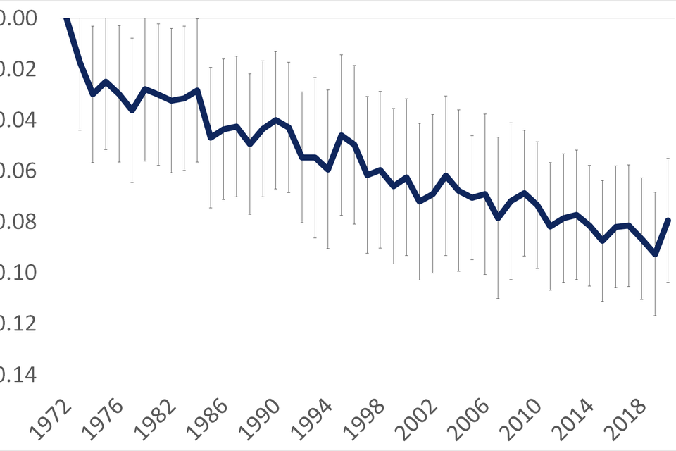
Source: Internal estimates based on The General Household Survey (1972 to 1992, 2005, except 1977, 1978), The British Household Panel Survey (1991 to 2008), the UK Household Longitudinal Study (also called Understanding Society, 2009 to 2020), the Taking Part Survey (2005) and the Labour Force Survey (2014 to 2020).

Note: The parameter shown is β from the log-multiplicative model lnF_ijk = μ + λ_i^O + λ_j^D + λ_k^C + λ_ik^OC + λ_jk^DC + β_kX_ij^OD where: F_ijk is a 3-dimensional contingency table giving origin i (O), destination j (D) and cohort k (C); μ is a scale factor; the first 3 lambda terms represent the effects of the distributions of individuals over origins, destinations and cohorts; the last 2 lambda terms represent the associations between origin and cohort (OC), and destination and cohort (DC); and finally the X term represents associations between origin and destination (OD), while β is a multiplicative parameter allowing these OD associations to strengthen or weaken over time. Odds ratios and model parameters are logged. Error bars show 95% confidence intervals around the estimates.

Limitations and gaps

There are many limitations of the index as it currently stands. The lack of harmonised education data across the UK is one of the most notable limitations. This is the case both for measures of educational drivers such as school quality and opportunities for further and higher education, and for intermediate outcomes such as social inequalities in attainment at age 16 years.

There is also a lack of local-level data for many of the intermediate outcomes and final social mobility outcomes. In order to obtain local area data, it is necessary to use administrative data in order to have sufficient sample sizes. Such data is available for some educational outcomes, although not harmonised across the UK, but are not in general available for labour market outcomes such as unemployment or earnings. While there is administrative data at a local authority level on the labour market, these do not include any measures of socio-economic background. Therefore they cannot be used to monitor social inequalities in outcomes.

A promising development is the linked administrative data of the Longitudinal Education Outcomes dataset. This includes a basic measure of socio-economic background as well as some labour market outcomes, such as earnings. While there are some limitations to this dataset, a priority will be to address these and to carry out similar data linkage exercises for the other nations of the UK.

Measures of socio-economic background in the administrative datasets lack granularity, and may be misleading when comparing areas with very different socio-economic profiles. The lack of granular data on socio-economic background in higher education statistics is also a concern. Conclusions are sometimes reduced to over-generalisation or comparing one group versus all others (such as those on FSM versus all others) simply because that is the best current data allows for. As more granular data on socio-economic background becomes available, this index should be adjusted.

Finally, a major limitation is the lack of good quality, regular data for monitoring income and wealth mobility. Other countries have linked parent and child administrative data. Expensive long-term panel studies are needed for this kind of research, and while the UK does have a rich tradition of such panel studies, it is of great importance to ensure that the tradition is maintained and refreshed, in the absence of administrative data. It would also be valuable if existing resources such as the LFS and the Wealth and Assets Survey could include additional measures on parental circumstances.

1. While described as a measure of free school meals (FSM) eligibility. FSM only includes those who have both applied for and been deemed eligible by the relevant local authority. It excludes an unknown number of people who might have been deemed eligible had they applied, and also includes many families who are relatively affluent. For more detailed discussions see, Graham Hobbs and Anna Vignoles, ‘Is children’s free school meals ‘eligibility’ a good proxy for family income?’, 2009. Published on TAYLOR AND FRANCIS.ONLINE.COM; Ioana Sonia Ilie, Alex Sutherland and Anna Vignoles, ‘Revisiting free school meal eligibility as a proxy for pupil socio‐economic deprivation’, 2017. Published on BERA-JOURNALS.ONLINELIBRARY.WILEY.COM; Daphne Kounali, Tony Robinson, Harvey Goldstein and Hugh Lauder, ‘The probity of free school meals as a proxy measure for disadvantage’, 2008. Published on BRISTOL.AC.UK. ↩

2. ONS’s 3-part schema (or model) of occupational class, used by the Social Mobility Commission. ↩

3. Self-employed and doesn’t have employees. ↩

4. Many occupations that would be classified as NS-SEC7 can instead fall into NS-SEC4 if the worker is self-employed. ↩

5. Office for National Statistics, ‘Labour Force Survey weighting methodology’, 2021. Published on ONS.GOV.UK. ↩

6. Office for National Statistics, ‘Adults aged 19 to 25 years who have undertaken job-related training or are in education, UK, July to September 2002 to 2021’, 2022. Published on ONS.GOV.UK. ↩

7. Office for National Statistics, ‘Rates of economic activity, unemployment, education and pay for specified age groups, UK, July to September 2002 to 2021’, 2022. Published on ONS.GOV.UK. ↩

8. Department for Education, ‘Early years foundation stage profile results: 2018 to 2019’, 2020. Published on GOV.UK. ↩

9. Department for Education, ‘National curriculum assessments at key stage 2 in England, 2019 (revised)’, 2019. Published on GOV.UK. ↩

10. UK Government, ‘Academic year 2020 to 2021 key stage 4 performance’, Published on GOV.UK. ↩

11. DfE has published more details regarding the methodology. See, Department for Education, ‘Statistical working paper measuring disadvantaged pupils’ attainment gaps over time (updated)’, 2015. Published on GOV.UK. ↩

12. Office for National Statistics, ‘Rates of economic activity, unemployment, education and pay for specified age groups, UK, July to September 2002 to 2021’, 2022. Published on ONS.GOV.UK ↩

13. Weighted according to sample size. ↩

14. Office for National Statistics, ‘Earnings and hours worked, place of work by local authority: ASHE table 7’, 2021. Published on ONS. GOV.UK. ↩

15. UK Government, ‘Create your own tables’. Published on STATISTICSSERVICE.GOV.UK. ↩

16. Office for National Statistics, ‘Rates of economic activity, unemployment, education and pay for specified age groups, UK, July to September 2002 to 2021’, 2022. Published on ONS.GOV.UK ↩

17. The Consumer Price Index (CPI) is a headline measure of inflation - the rate at which prices increase. This is calculated by the ONS who track the changes in prices for a basket of goods representing the average consumer. For more information see the ONS website: https://www.ons.gov.uk/economy/inflationandpriceindices ↩