
A Bite-Sized Guide to Visualising Data
Published 10 November 2022

© Crown copyright 2022
This publication is licensed under the terms of the Open Government Licence v3.0 except where otherwise stated. To view this licence, visit nationalarchives.gov.uk/doc/open-government-licence/version/3 or write to the Information Policy Team, The National Archives, Kew, London TW9 4DU, or email: psi@nationalarchives.gov.uk.
Where we have identified any third party copyright information you will need to obtain permission from the copyright holders concerned.
This publication is available at https://www.gov.uk/government/publications/a-bite-sized-guide-to-visualising-data-a-dstl-biscuit-book/a-bite-sized-guide-to-visualising-data
Foreword
“What is the use of a book”, thought Alice, “without pictures or conversations?”, so said Alice during her adventures in Wonderland. In this little Biscuit Book you will get conversations (sort of) but the main focus is about pictures, or more precisely visualisations of data; there’s a hint in the title. Data by itself is pretty boring. Staring at a list, or worse still, a table of numbers, is not most people’s idea of a good time. And, it can be difficult to interpret quickly. Explaining the data in text can be better but can still be difficult to understand. Stories and conversations are better, and adding images or visualisations is even better.
This little book presents a number of popular (and indeed less popular) ways of visualising data, and explains their strengths and weaknesses. It is intended for those interested in producing visualisations and more so for those who need to understand them.
Siân Clark, Corinne Jett, Toni Emery, Glen Hart, Jamie Lendrum
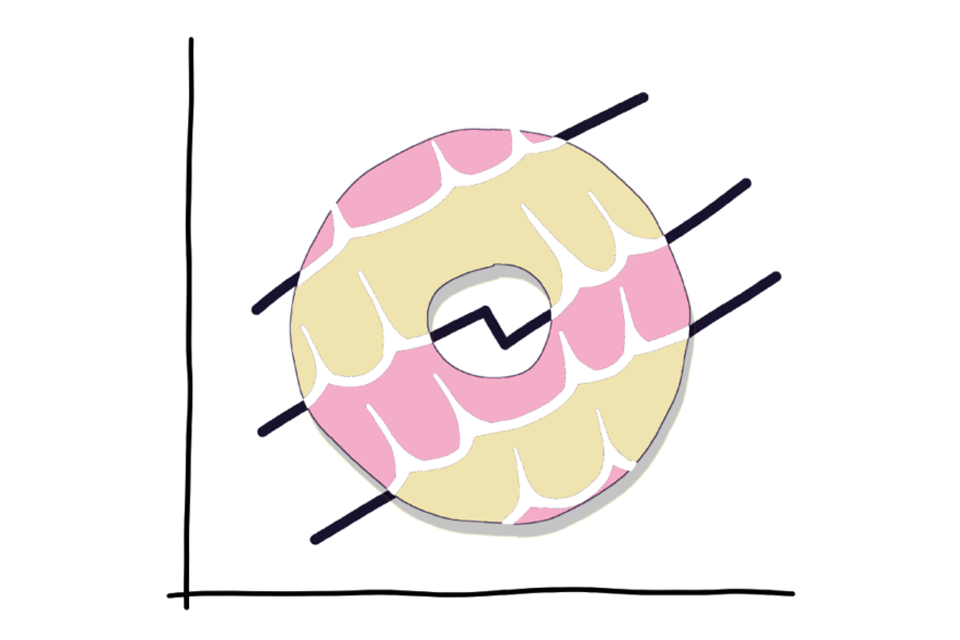
Cover image - an iced ring biscuit on a graph.
What are visualisations?
Data is usually encountered as a bunch of numbers, sometimes a rather large amount of them. This can make understanding what it all means a bit of a challenge. Data can also come in the form of huge quantities of text, images, and more. Sometimes we use data visualisations to bring out the important messages that may be hidden behind the mass of numbers and information. If you’ve seen diagrams and graphs before, these are what we mean by data visualisations.
You probably see data visualisations in your everyday life without even realising that’s what they truly are. These visualisations are meant to convey important and useful information to the user in a quick and easy way. Below are a few good examples you may see regularly.
Nutritional information
Found everywhere in supermarkets across the UK today, a traffic light data visualisation was introduced by the Department of Health in 2013 to help people understand the complicated nutritional information on the back of food packets. Instead, you can now read a simpler colour-coded label that highlights the key nutritional information with the aim of making it easier for you to make healthier food choices.
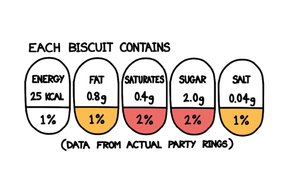
A graphic of a typical nutritional information label.
(Perhaps give this one a miss next time you go to grab your favourite biscuit!)
Fuel gauges
A fuel gauge (or dial) is an instrument used to indicate the amount of fuel in a fuel tank. The pointer and level notches on the dashboard create a simple and effective visualisation that let the user know how much fuel they have left in their vehicle. Most fuel gauges look similar, with some having F for Full and E for Empty and other having 1 and 0 for the same levels respectively. Imagine having to use a car without one of these!
The impact that a visualisation makes is dependent on the poor hapless souls upon whom it is inflicted, and their ability to understand what they are looking at. The ways we can visualise data can be complex and require the viewer to have a high level of understanding. This isn’t great, but it may be necessary due to the need to explain complicated information. We try to combat this in this Biscuit Book by providing a clear caption with each visualisation we show. We hope this will help you understand each one regardless of your prior knowledge.
To help us bring visualisations to life, we conducted a survey on a very important topic. We got almost 200 people to tell us:
What is your favourite biscuit?
Below we will provide a short summary on what to look for when reading a visualisation to ensure you give yourself the best chance of understanding, no matter how complex the visualisation seems. We will use the survey results to create a visualisation that shows which biscuit was most popular:
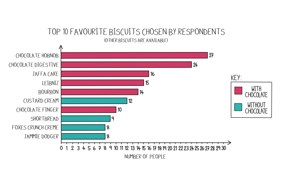
A bar chart depicting the popularity of a range of biscuits demonstrating that the inclusion of chocolate makes them much more favourable with scientists.
A survey was conducted by Dstl in Winter 2021 that asked “What is your favourite biscuit?”
The visualisation shows the top 10 favourite biscuits chosen by respondents from a set list, and categorises them by chocolate or not.
-
Begin with the title, an obvious place to start. The title should offer a good description or a takeaway message to help you understand what is being presented (but don’t be surprised if the title is vague or doesn’t exist!).
-
A caption and title will offer more detail, usually including what data is being used, where the data has come from and any formatting choices like colour or shape legends if not mentioned elsewhere (again, suppress your surprise if the caption is not great or missing!).
If the visualisation contains both of the above then you are doing well. If not, you need to be extra careful when it comes to interpreting the content and you may not understand what is being presented. You can use what you’ve learnt from the title and caption to cross-reference against each axis. We call the horizontal line the x-axis and the vertical line the y-axis. In this example we can see the number of people (along the horizontal x-axis) that chose which biscuit (up the vertical y-axis) as their favourite. In this diagram, we have also coloured the bars by whether the biscuit is chocolate flavoured or not, and you can see the corresponding colour in the key or legend.
A bar chart depicting the popularity of a range of biscuits demonstrating that the inclusion of chocolate makes them much more favourable with scientists.
A survey was conducted by Dstl in Winter 2021 that asked “What is your favourite biscuit?”
The visualisation shows the top 10 favourite biscuits chosen by respondents from a set list, and categorises them by chocolate or not.
Let’s look at the top bar coloured in pink. We see it is lined up on the y-axis with Chocolate Hobnob. If we trace where the bar ends along the x-axis, we see it matches the label of 27 people. Therefore, we can deduce that 27 people chose a Chocolate Hobnob as their favourite biscuit.
In this instance, we have displayed the survey information in a horizontal bar graph. There exists so many different types of data visualisations, some of which are shown on the next page in our Visualisation Bestiary.
Visualisation bestiary
A bestiary is a collection of beasts (and believe us, some visualisations can be real beasts).
Bar Chart
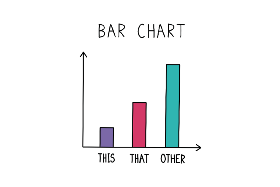
Example bar chart
Compare quantities of different things.
Pie Chart
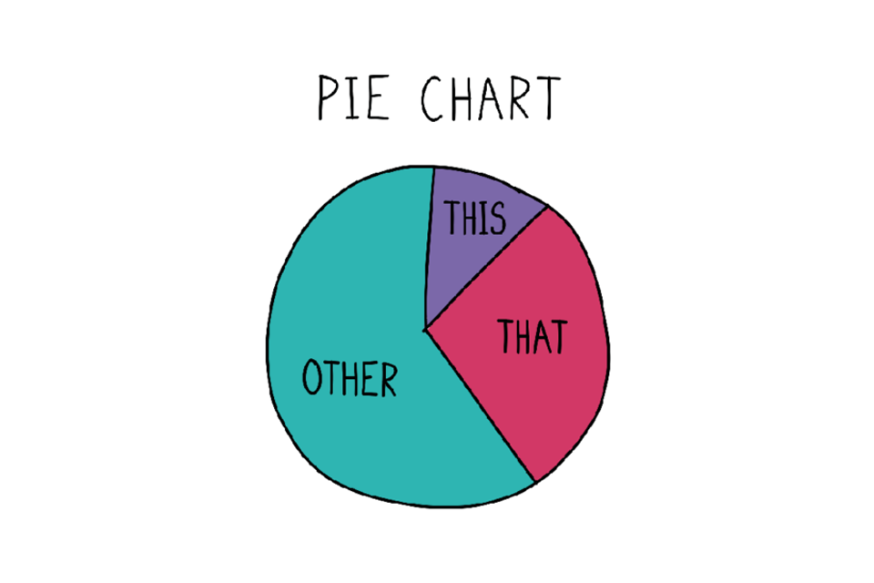
Example pie chart
Show percentages of a whole.
Donut Chart
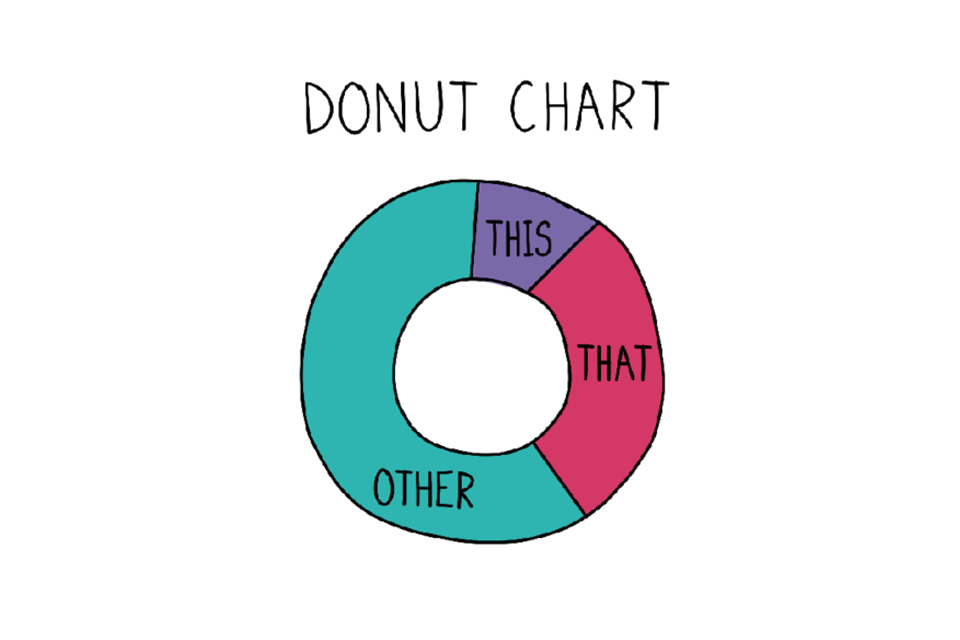
Example donut chart
Show percentages of a whole with an added hole!
Spine Chart
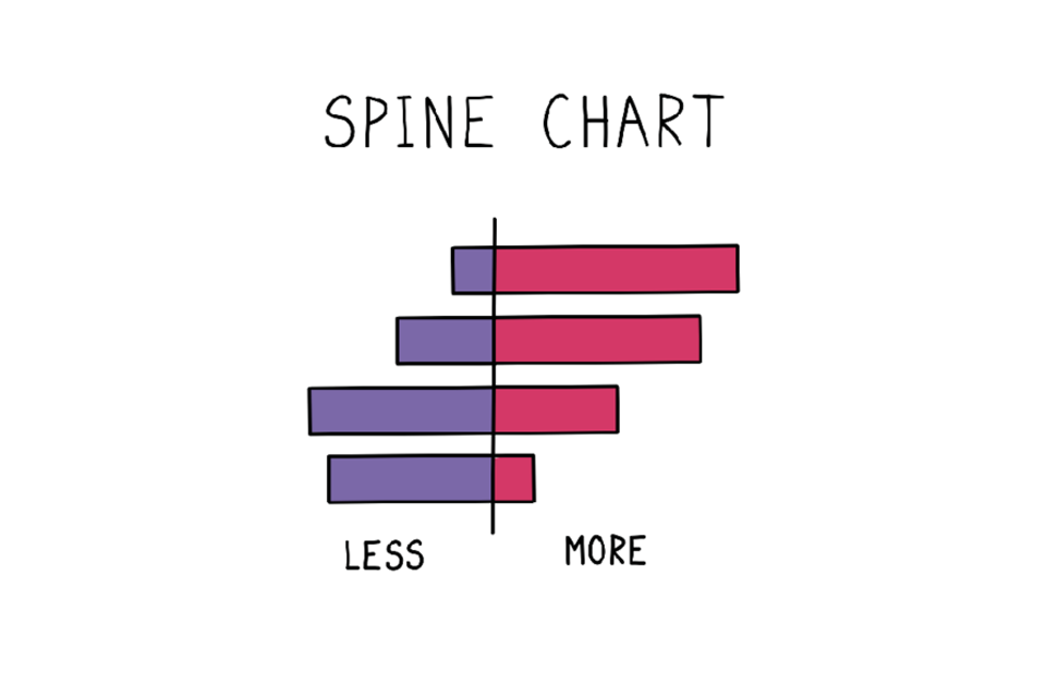
Example spine chart
Compare two groups across different measures.
Lollipop Graph
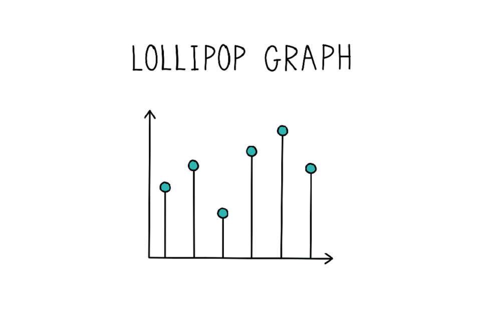
Example lollipop chart
Numerically compare different groups. This is really a snazzy Bar Chart.
Waffle Chart
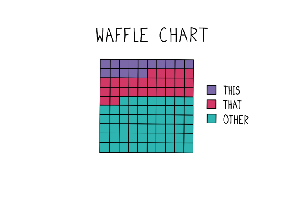
Example waffle chart
Show percentages of a whole. In spite of its name these are not usually edible.
Area Graph
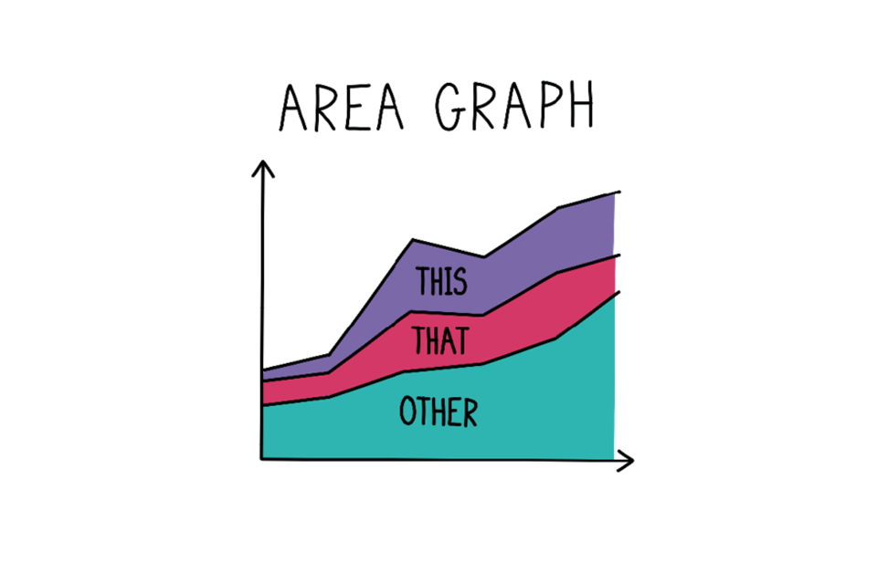
Example area graph
Compare relationships over time.
Scatter Plot
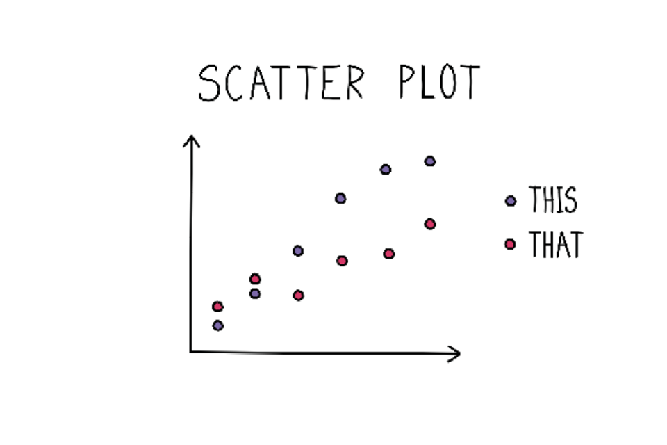
Example scatter plot
Compare relationships between pairs of data.
Bubble Chart
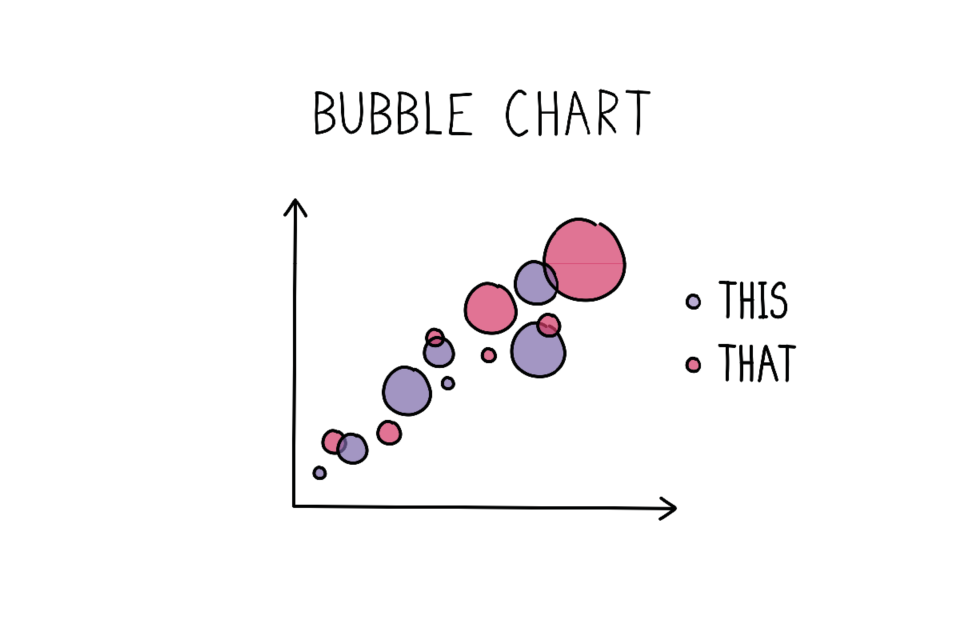
Example bubble chart
Compare relationships between three variables.
Line Graph
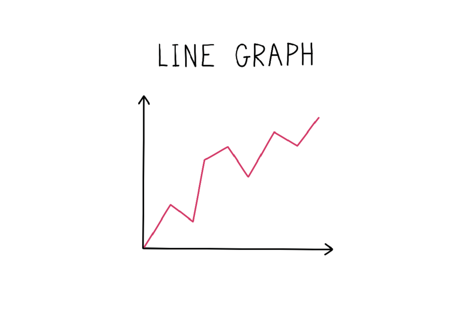
Example line graph
Track changes over a period of time.
Choropleth
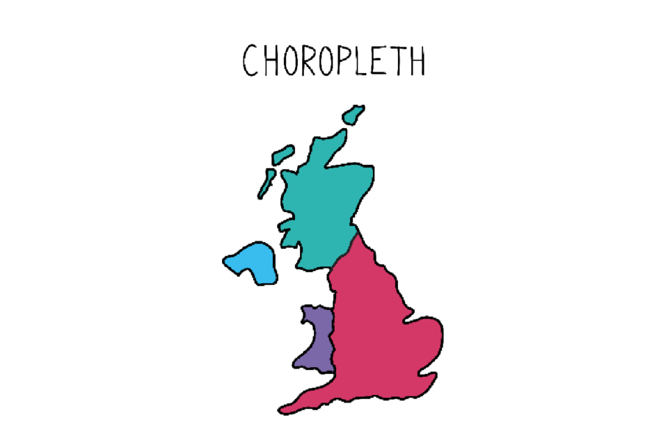
Example choropleth
Show differences in geographical regions.
Wordcloud
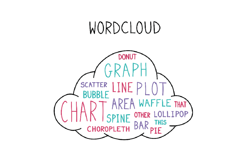
Example word cloud
Display most popular word in a body of text.
Lies, damned lies and visualisations
Misleading people with graphs is not a new problem; mostly this is done unconsciously or just because the visualisation is poorly described, or designed. Sometimes, it is deliberate. In fact, it is so easy to mislead people with statistics and charts that Darrell Huff wrote a book called How to Lie with Statistics in 1954 (that’s nearly 70 years ago at time of writing). So why might people mislead and how may it manifest itself? Read on!
Motivation
Why would somebody try to mislead you with a visualisation? There are two main reasons:
-
They don’t mean to – they are just mistaken;
-
They want to influence you in some way because:
They want you to buy their product;
They want you to subscribe to their beliefs, which may be wrong;
They have been paid by somebody else in aid of the above.
If you see a visualisation saying ‘sweets are good for your teeth’ and you know it was published by a sweet manufacturer, you would be justified in being somewhat more suspicious than if it had been published by your dentists, and even then you still might want to change dentist!
Correlation and causation
So why do people develop mistaken beliefs? People are hardwired to look for patterns and trends. This is why we have so many conspiracy theories. While it may seem silly to most people to believe that the elite are in fact space lizard monsters in disguise, there is so much evidence!
Two important words to know here are correlation and causation:
-
Correlation: there is a statistical association between things;
-
Causation: one thing changing is causing the other thing to change.
You might have heard the phrase ‘correlation does not imply causation’ but what does this actually mean? Because we humans are so good at spotting patterns and trends, sometimes when people see two lines match on a graph (because there is a correlation), they might assume one thing is causing the other to happen (because there is causation).
However, this is risky and can lead to mistakes. For example, you may note that when windmills are rotating, there is lots of wind. As a result, you may infer that the turning of the windmills is causing the wind to blow. In this case, your common sense will tell you that this is incorrect – the wind is what moves the windmill, so there is causation – just the other way around (which is good news for the windmills). Sometimes it is less straightforward than this, and people can get so wrapped up in their message or story that they miss the obvious, so make sure to keep your eyes open!
As well as mixing up the cause and effect (such as with wind and windmills), sometimes two lines on a graph may seem to line up, showing correlation (basically one increases as another increases, such as wind speed and speed of windmill rotation).
However, there are many cases where things may look related but they (probably) aren’t! Some well-known examples of these include correlations between:
-
Total per capita consumption of cheese in the US and the number of people who died by becoming tangled in their bedsheets (2000-2009);
-
Number of people who drown by falling into a swimming pool and the number of films Nick Cage appears in (1999-2009);
-
Worldwide non-commercial space launches and sociology doctorates awarded in the US (1997-2009);
-
Autism rate and organic food sales (from 1998 to 2007);
-
Internet Explorer market share and US murder rate (from 2006 to 2011).
Having said these are all coincidences, there is a small chance that there really may be a link but for reasons that we cannot yet fathom. To be safe, it’s best to assume that correlation does not ALWAYS imply causation and think about the motivations of whoever is trying to prove the causation – have they only selected SOME of the data that lines up nicely and missed out the parts that don’t? It’s up to you to decide on the context and whether a link makes sense (and it can be really interesting and fun to think about!)
Sneaky axes
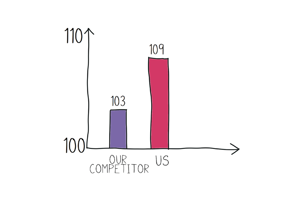
Sometimes people want to make a difference look bigger than it really is. You might have seen something like this in the news or a business report…
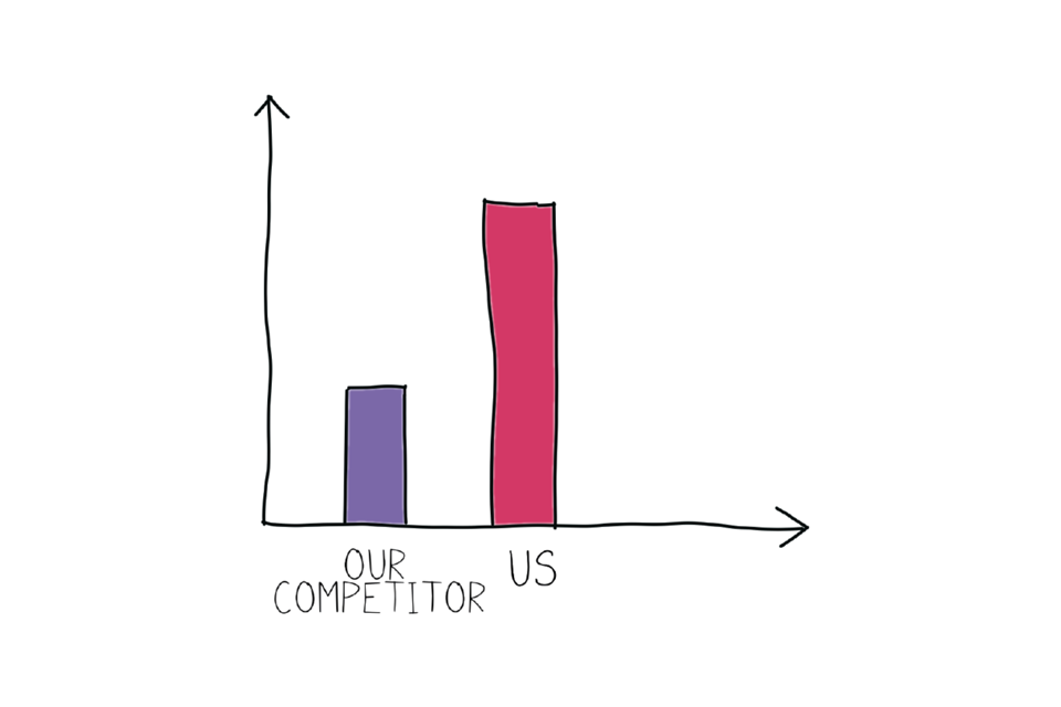
Example bar chart that is slightly deceiving.
An unlabelled bar chart showing how much bigger our bar is than our competitor’s.
As you can see, we have a much bigger bar than our competitors! …Or do we? You might notice a distinct lack of numbers on this graph. If it were properly labelled, it could look like this:
Example bar chart that puts the results into proportion.
A labelled bar chart showing that while our bar looks bigger, the difference in ‘score’ is actually quite small
The y-axis (that’s the vertical one) starts at 100, and only goes up to 110. If we add data labels to the bars, you’ll see that our competitor’s figure (103) is not so different to ours (109). While it is technically ‘OK’ to show a y-axis like this, it can be misleading and hide anything that is happening below the minimum point. To present this more honestly, in most cases the y-axis should start at 0, and end at an appropriate number. Here’s a more honest representation:
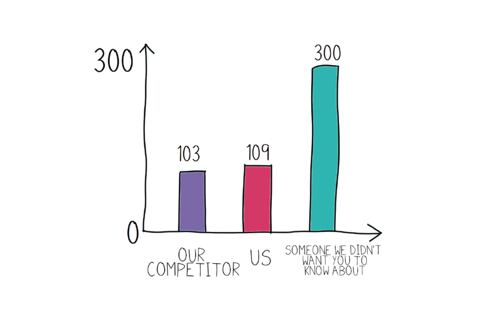
Example bar chart that tells the whole story.
A labelled bar chart showing that our bar is very close in size to our competitor’s, and that in the grand scheme of things, both of us have a much smaller bar than another competitor we didn’t want you to know about.
So not only are we not as far ahead of our competitors as the original graph made it look like, we have also lied by omission (basically we didn’t technically ‘lie’, but we didn’t mention something important and relevant because it didn’t suit us) by not including our other competitor, who has a much a bigger bar than us.
Another issue can be multiple y-axes. They can be useful to show things when two sets of data are related but not on the same scale (for example, height in metres vs height in centimetres). This may not deliberately be misleading, but it can definitely be confusing! Let’s say we want to plot some data that look like this:
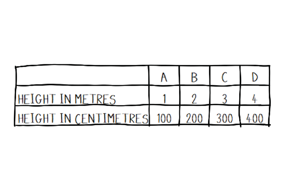
A table showing different heights each in metres and centimetres.
A table showing the relationship between height in metres and centimetres at four separate points.
Pretty similar, right? If you are 1.5 m tall, you will also be 150 cm tall, that’s not going to change. Meanwhile, if we plot this on a graph:
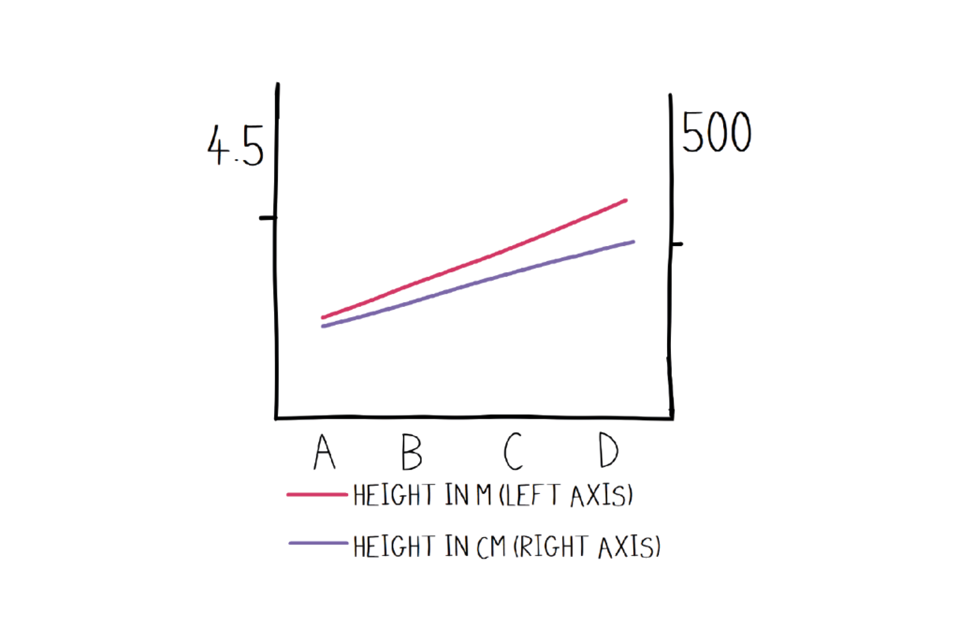
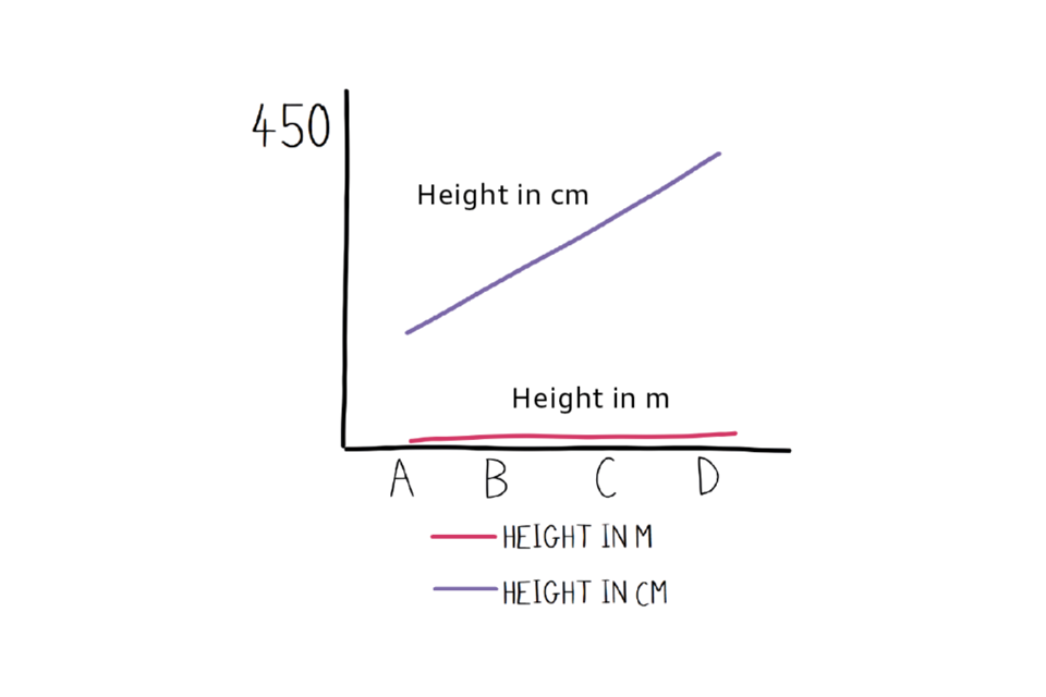
A misleading graph.
A misleading labelled graph with two axes showing height in metres (left) and centimetres (right). Because the axes are not synchronised, it looks as though height in metres (1, 2, 3, 4) is greater than height in cm (100, 200, 300, 400)
We’ve made it look like the purple line (height in centimetres, from 100-400) is smaller than the red line (height in metres, from 1-4). However, the purple line should be compared to the right hand axis and the red line to the left, and we’ve been extra sneaky and made the axes not match up (they are ‘unsynchronised). In fact, if they were using the same axis, they’d look something like this:
Another misleading graph.
A labelled graph with one axis representing ‘height’ but with no units.
We can play with the aspect ratio to make this even more confusing by adding some extra, unused, categories on the x-axis:
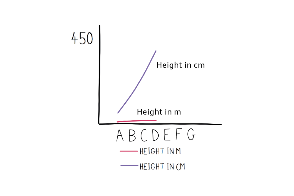
One more misleading graph.
A labelled graph with one axis representing ‘height’ but with no units , and some unused categories (E, F, G) that compress the rest of the graph and make one of the lines appear very steep.
We’ve made it look like the purple line is growing really sharply relative to the red line when it isn’t really. There are all kind of tricks that can be played with perspective. It’s generally best to check the numbers and look for anything extra that might be confusing things.
The legend of context
For visualisations, context is everything. Take a look at the ‘thermal image’ below:
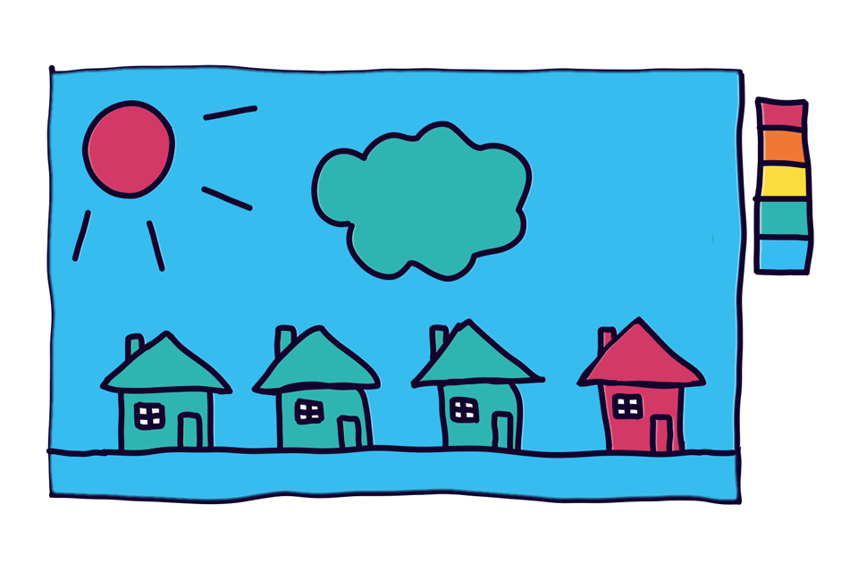
Example heat map showing one hot house, but being unclear how hot compared to adjacent houses?
You may often see heat maps like this and just know that red is ‘hot’ and blue is ‘cold’. With this instinct, it looks like the house on the far right is very ‘hot’ compared to the other houses on the street. However, we are lacking some important information – the context in the legend. If the coolest colour (blue) represents 20°C the hottest colour (red) represents 21°C, then a very small change looks very big. Alternatively, if the coolest colour represents 20°C and the hottest represents something much warmer at 40°C, you may begin to question what is actually going on in the house on the right …
Subjective scaling
There are two key aspects to this trick:
-
People are not very good at judging the size of things, particularly if they already have an idea of what they’re expecting to see;
-
If one-dimensional data (such as ‘length’) is represented by 2-dimensional visualisations (such as area), they won’t scale in the same way.
Here’s a simple example. We want to show how size changes when we count 1, 2, 3:
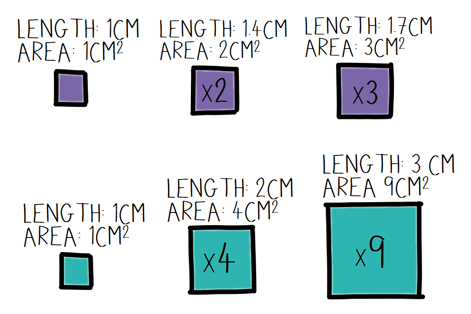
Example chart showing the problems associated with scaling.
In this example, the top option increases the area in line with the sequence 1, 2, 3. However, the lower option increases the height and width of the square in line with 1, 2, 3. This means that the area actually represents 1, 4, and 9. Here lies the problem with using area to represent a number which is 1-dimensional.
And what would you think if we took the labels off, and primed you with the expectation that we’d see enormous increases from 1 to 3? You’d be better off showing this with a simple line or bar chart.
The problem with pies
The problem above continues with pie charts. Pie charts are one of the most popular and familiar visualisations, but there are many places where they shouldn’t really be used. Don’t get us wrong, pie charts can be used in a correct way; they can be used to show a very clear split between very clear categorical proportions (for example halves, thirds or quarters). However, pies can be particularly prone to problems.
A matter of perspective
Have you ever seen a 3D pie chart? Sure, the author might have thought it would add some ‘wow factor’, but the perspective can be very misleading.
We promise you that the two charts below show the same data. On the right, the slices that face forwards may appear larger than the slices that are facing further away. However the chart on the right, which shows the exact same data, makes it clear that each slice is actually the same size!

Two example pie charts showing how adding perspective can alter perception.
Too much to show
Too many categories on one pie can make it unreadable.
Take a look at the pie chart below. Information overload, right?! Good luck working out what it means, let alone matching that many colours to the legend underneath (especially as some are duplicated, so you have to sort of follow them around the pie).
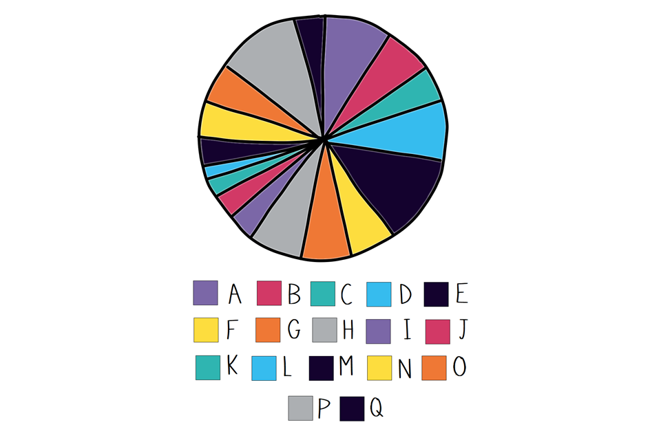
Example pie chart with too many segments.
The end result is that the pie fails to communicate its message effectively, so you’ll have to look elsewhere to understand the message. Just thank your lucky stars it wasn’t 3D as well!
Just plain wrong
Some pie charts add up to more than 100%, and this is a bit rubbish. Sometimes, this can happen when people give more than one answer to a survey and this is counted in the data. Sometimes it is a rounding error, and sometimes people just plonk a % symbol on the end of a number rather than actually calculating anything. So please do add up any values you see on a pie chart to make sure they make sense!
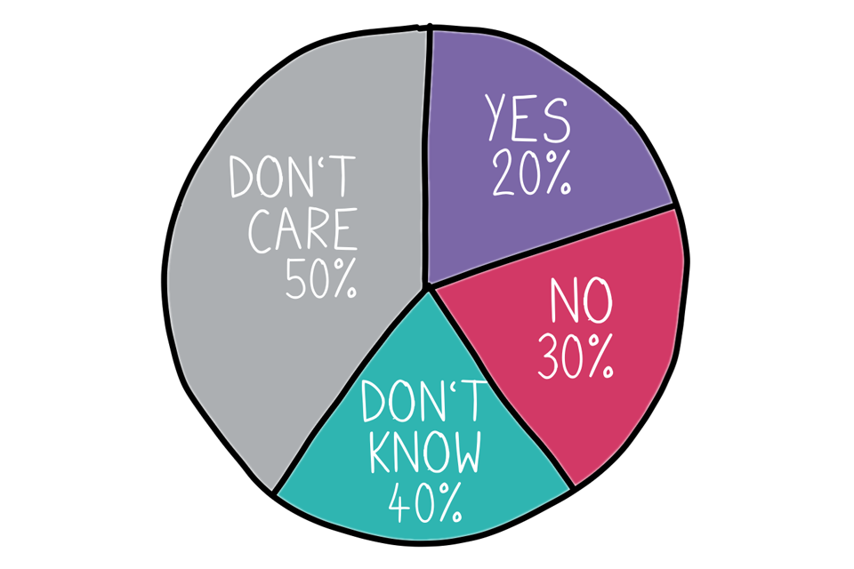
Example pie chart that doesn't add up.
Spotter’s guide
To summarise the chapter, please see this handy spotter’s guide for dodgy graphs and charts. If many of the warning signs below appear, double check the graph and ask questions. It doesn’t necessarily mean someone is trying to mislead you, but it’s worth approaching any conclusions drawn from such graphs with scepticism.
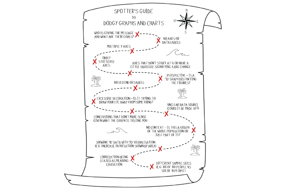
A guide to inaccurate graphs and charts drawn to look like a pirate's treasure map.
Look out for:
- who is giving the message and what are their goals?
- no axes or data labels
- multiple Y-axes
- oddly stretched axes
- axes that don’t start at 0 or have a little squiggle signifying a big change perspective - is a ‘3D’ graph distorting the figures?
- no legend or labels
- excessive decoration - is it trying to draw your eye away from something?
- unclear data source (could it be made up?)
- conclusions that don’t make sense given what the graph is telling you
- no context - is this a graph of the whole population or just a part of it? showing ‘1D’ data with ‘2D’ visualisation (for example increase in inflation shown by area)
- correlation being stated as meaning causation
- different sample sizes (for example 10% of 100 people versus 50% of 10 people)
Mostly maps - visualising geographic information
The most common way to visually represent locational and geographic information is through the use of maps. However, maps can lie too! They can lie in a number of ways without intending to do so, but this does not mean that maps are of no use. Far from it in fact, it just means you need to be aware of how they have the potential to mislead. Geographical information can be represented in other ways, for example a bar chart could be used to compare city populations. But, in almost all of these cases, you lose the spatial relationships. Therefore, in this section we will deal only with maps.
Projections
The World is basically a sphere (flat-earthers might want to skip this whole section). As spheres go, it’s not a terribly good sphere. But for this Biscuit Book we’ll skip the fact that it’s slightly flattened, chubbier around the equator and has lots of lumps and bumps. This still leaves the problem that you will usually have to represent a sphere on a flat surface. This is a process known as projection, where a sphere is projected onto a flat surface in some way, but this can’t usually be done without causing some distortion. There are many different ways of doing projections – too many for a Biscuit Book. The one we are most familiar with is the Mercator projection, as it is most frequently used to represent maps of the whole Earth. In this representation, the further north or south you go, the more stretched the map is. So you need to be aware of such distortions. For maps of relatively small areas, such as a town, you don’t have to worry about such distortions. But for large areas, it’s important to understand what projection has been used and how it distorts the base map.
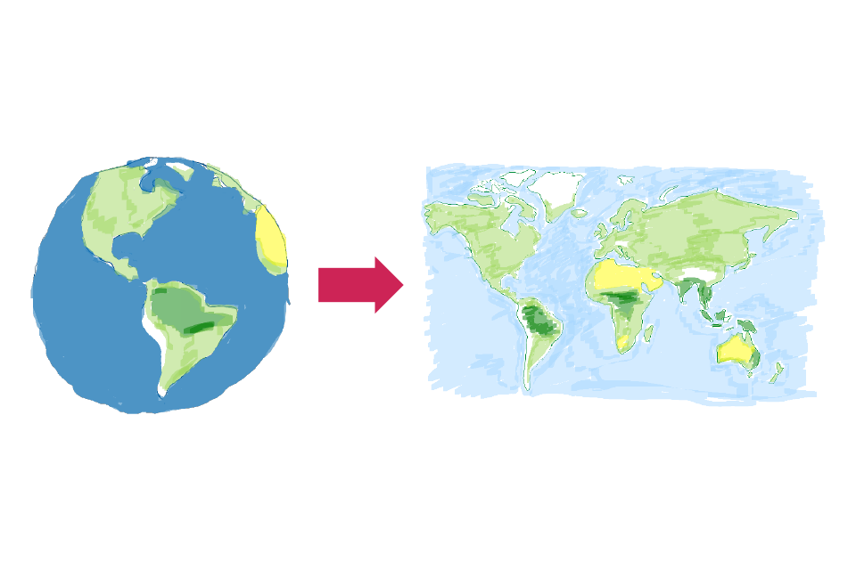
The world projected as a map with associated distortions.
Turning a sub-standard sphere (The Earth) into a flat map
Common types of map
Contour map
Contours are lines which represent a characteristic that has the same value along the whole line. Usually, values are shown with fixed steps between them. Popular uses for contour lines include equal height or elevation on Ordnance Survey maps, or lines of equal atmospheric pressure on weather maps. The example below shows terrain height at 10 metre intervals. Note that you can’t assume a steady progression from one contour line to the next, although this is often the case.
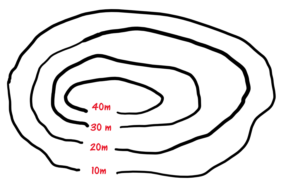
Contour map
Choropleth maps
A choropleth map uses colours to represent different values of something by area. Imagine a map that shows annual biscuit consumption by county. A choropleth map will categorise quantities of consumption, and then use different colours to represent these categories by county. For example, blue could represent 0–10 million biscuits, yellow is 10–20 million, green is 20–30 million and red more than 30 million. This looks nice, but can have problems when smaller areas are easy to miss, or look less important when compared to larger areas.

Choropleth map
Proportional symbol maps
Proportional symbols represent values by size of a symbol, where the larger the symbol (usually a circle), the larger the value. So in the case of biscuit consumption, we could show highest consumption values by county, with each county represented by a symbol sized to represent the peak consumption value. One issue with this type of map is that you have to choose a representative point to place the symbol, so symbols can sometimes overlap and make the map more difficult to interpret.
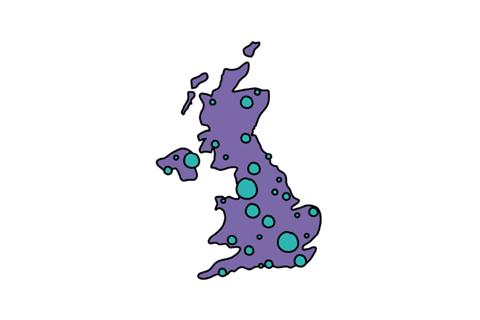
Proportional symbol map
Cartograms
A cartogram is a type of map where areas with certain values are shown in proportion to the area that the value represents. This is best seen through an example and it makes familiar maps look a bit weird! For example a map of global poverty will expand areas like Africa, but shrink areas such as the Americas and Europe. Cartograms are also known as anamorphic maps.
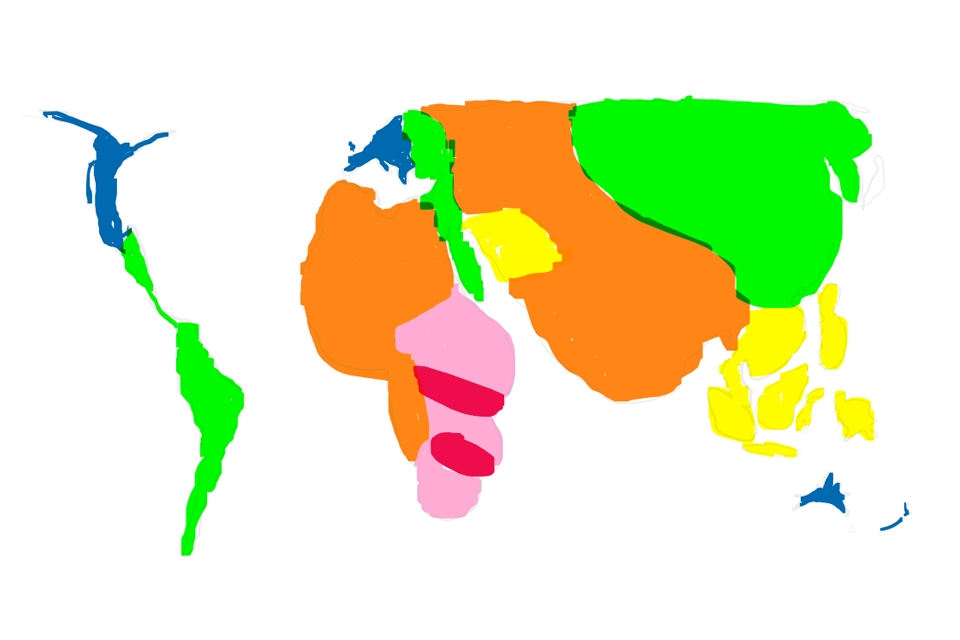
Cartogram
Dot density
Dot density maps show spatial patterns through the distribution of dots. These dots represent related things, for example the distribution of people whose favourite biscuit is a chocolate digestive. Different coloured dots or different symbols can be used to represent different things, so we could compare the distribution of chocolate digestives against jammy dodgers or hob nobs.

Dot density map
Heat map
A heat map is a visualisation that uses graded colour to represent the intensity of something over an area of interest. An early use of this technique was to show the height of terrain, but there are many other possible uses. One thing to watch out for with this type of map is the scale or legend. For example ‘red’ may look much hotter/more intense than blue, but if red represents an average of 10 biscuits a week and blue represents 9, then the difference is not as big as the colour change makes it look.
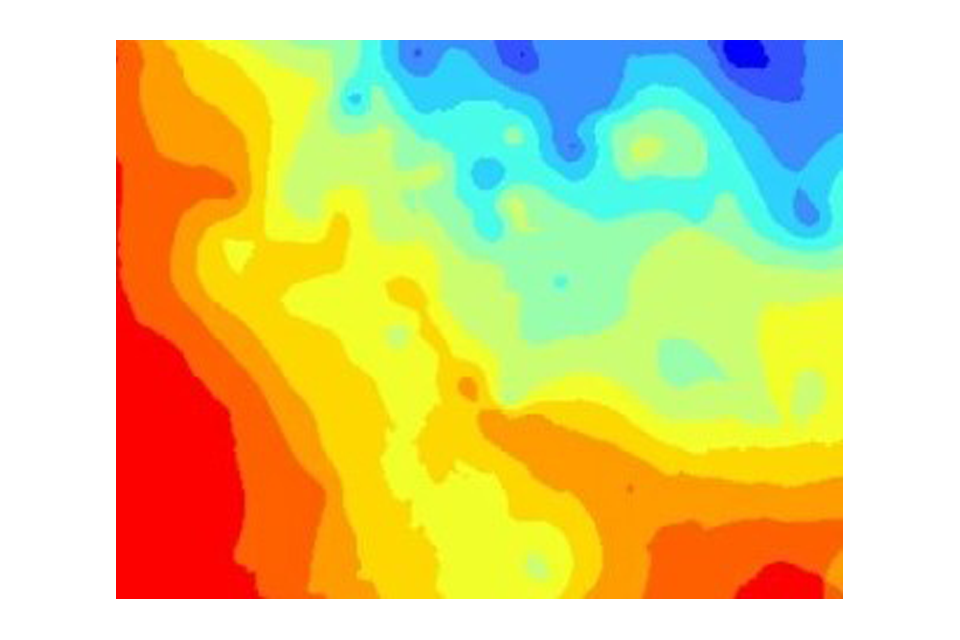
Heat map
The problem with boundaries
Map-based visualisations often use data that is represented against areas that group data by boundaries constructed to simplify things, like administrative areas (think counties, postcodes and things like that). These boundaries do make it easier to show, for example, biscuit preferences by British county. However the problem with administrative boundaries (and similar) is that they may not properly reflect the optimum way the data could be represented. Quite often, the biggest differences appear to occur across boundaries, even though a closer examination of the data will show this not to be the case. They can also mean that the data was collected differently in each area and so may not be directly comparable. As an example, it has been difficult to compare Covid cases across different countries because the data is collected differently by each country. The general rule is be aware of what differences can occur between data shown against artificial areas such as administrative areas.
Dashboards
Whilst many visualisations might find their home in a report or presentation, some can be embedded in something we call a dashboard. We see dashboards everywhere in everyday life in some form or another, and some are more elaborate than others. The stereotypical dashboard is one you might find in a car – it updates as you change speed, use fuel, and you can sometimes choose what type of driving data you see (depending on how fancy your car is).
A data dashboard is defined as:
“A type of graphical user interface (GUI) that provides a centralised, repeatable, and possibly interactive means of visualising and summarising insights from datasets. It can link to static data (such as a csv) or ‘live’ data that will continually update (for example via APIs).”
Well, that’s a fancy definition! A simpler one is …
… a dashboard is a way to group together a number of related visualisations. The user may be able to interact with them in some way and they may be up-datable.
This is what a typical dashboard may look like:
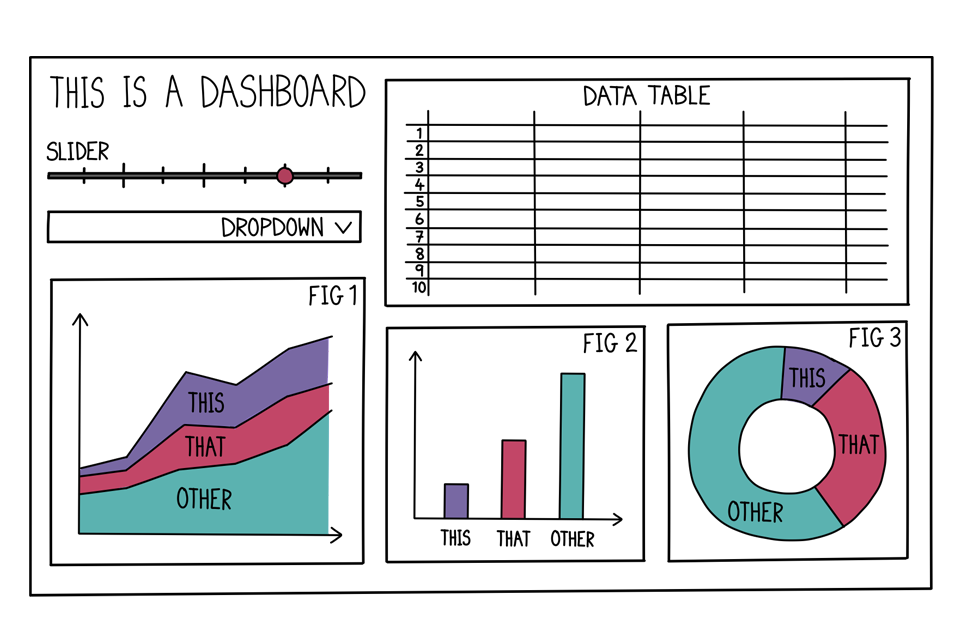
Example dashboard
A single visualisation can tell a short story by itself, but a dashboard can provide a much richer narrative. It can look at an issue from different perspectives and can allow you to dig deeper into why something may be happening.
Dashboards should be intuitive and easy to use, whether you’re a boffin or not. They should provide a “single source of truth” that is updated automatically as the underlying data changes, ensuring everyone has an up to date understanding of the way things are.
However, dashboards are only as good as the data that drives them and the metrics and visualisations that have been chosen to be displayed. Just because it looks pretty or modern, it doesn’t mean that it’s reflective of reality. So how do you trust what a dashboard is telling you and use it to make decisions? Part of this comes with experience; if you deal with the same dashboard over time, you learn its strengths and limitations, but most importantly its fitness for purpose. The key thing to remember is to always ask ‘why’ for everything you see. The dashboard will show you the ‘what’, but the ‘why’ may be more elusive. The dashboard is often the kick-starter for conversations with people who know the data better than you do.
If you’re the person designing a dashboard, you should ask yourself the same sorts of questions as you do when you create a visualisation:
-
Who is it for? Why do they need it?
-
How will it be used? How often?
-
What set of visualisations can best tell the story?
Below we share some tips for creating intuitive dashboards.
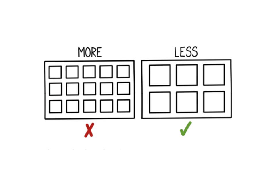
One of six Example dashboards
Only include what’s important
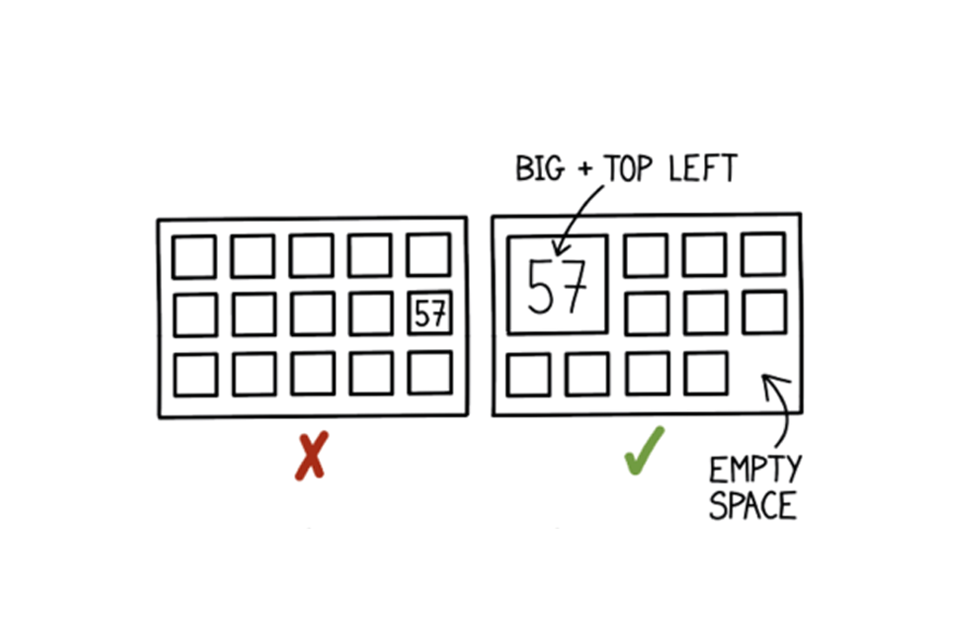
One of six Example dashboards
Use size and position to indicate importance
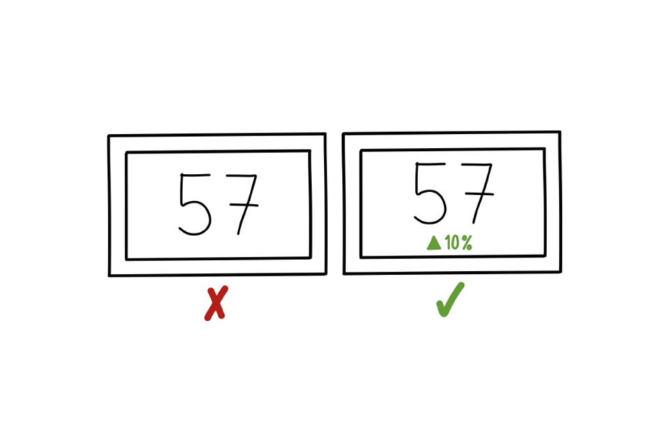
One of six Example dashboards
Provide context
One of six Example dashboards
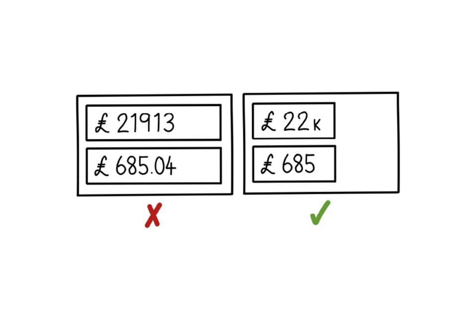
Round your numbers
One of six Example dashboards
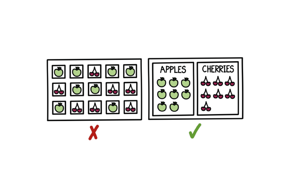
Group related metrics
One of six Example dashboards
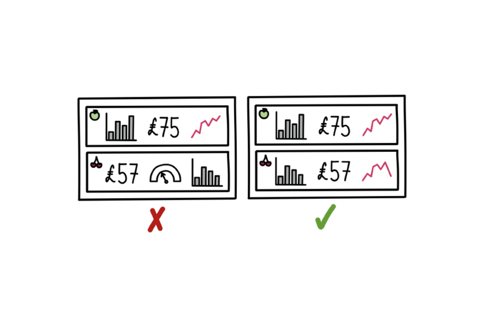
Be consistent
A little more unconventional
Sometimes it can be fun to make a visualisation that’s a little more ‘out there’. While there are many options for what you can do, here are a few of our favourite less conventional options.
Here are some examples:
-
Sankey plots;
-
Coxcomb charts (also known as aster plots or rotated histograms);
-
Sunburst charts (also known as circular bar plots);
-
Chernoff faces and fishes;
-
Treemaps;
-
Circular packing;
-
Dendrograms.
We won’t describe them all as now you have a name you can look them up, but there are many more options out there and sometimes people come up with really clever ways to show information. Keep an eye out!
While seeing an unusual visualisation can be exciting, there are pros and cons to using something different – accessibility considerations being an important one.
We’ll give one example in a little bit more detail (because we couldn’t resist it): Chernoff Faces (we’ll be honest, Chernoff Faces are so off-piste that you’ll see why we couldn’t resist). In a Chernoff Face, different characteristics are associated with different attributes of the data, and the value of the data alters the characteristic in the face. The example we have given shows a set of Chernoff Faces that explain different attributes about several biscuits. Each face shows you the price, weight, pack size and year of creation of a selection of different types of biscuit. As you can see, there are many elements to each face that explain what they mean, and it can be difficult to work out what is going on! Whilst it might be eye-catching and funny, and help you spot outliers (in this case the Party Ring looks a lot different to the others), and match similar faces (like the Bourbon and Ginger Nuts who have similar cost and weight), it requires a lot of context to explain and lots of thinking is needed.
When it comes down to it - how useful is it really?!
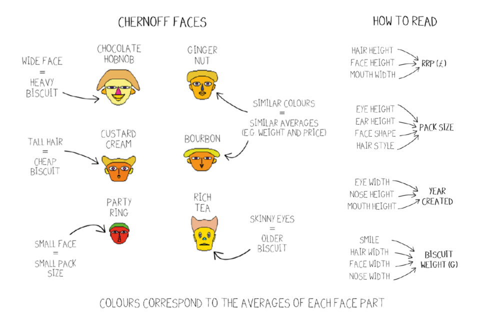
Examples of Chernoff faces
These faces were created using the Aplpack package in R.
Visualiser’s toolkit
Mostly this Biscuit Book is written for those that need to understand someone else’s visualisations. But, it’s worth putting something in for the analyst who will create visualisations to communicate their findings. It’s a bit meatier than what’s gone before in this book, but still less confusing than an article you may find online. So grab a couple more biscuits and get yourself a large mug of tea if you want to tackle this bit!
What, why and who for
When someone wants to make a visualisation, they will need to think about a number of things before they even consider whether to use a pie or lollipop chart.
What
First of all, it’s helpful if the author thinks about the visualisation from the perspective of a problem to solve, or a specific thing to achieve. This should focus on the end goal – this is what is important to communicate – rather than the specifics of what to include. So instead of “I want a pie chart of this and a bar chart of that”, they ideally say “I want to see a trend in the price of biscuits over time”. In this example, pie charts would be unlikely to be a good option. While this may sound easy, it can sometimes be quite complicated. One benefit though is that a title for the visualisation will naturally fall out of the description of the end goal!
Why
Next, it’s important that some thought is given to why the visualisation should be made – that is in the case above, why they want to show the trend in biscuit prices. This can help add extra insight or depth to the visualisation, or help reduce the scope to keep it focused to the story that needs to be told. In the example above, let’s say they want to show the trend to help people make decisions about which biscuits to stock up on. Knowing this will also give them the opportunity to link up to other information to provide a better narrative about the visualisation, such as the price of flour, stock prices, company mergers and so forth (because choosing biscuits is serious business!).
Who for
Next, it’s important they consider who the visualisation is for: the target audience. If the visualisation is showing biscuit prices over time to some university professors, it is likely to be very different to something showing biscuit prices over time to children, teenagers, or even politicians for that matter. Thinking about who the ‘vis’ is for helps with picking cosmetic details to use or avoid. Having said this, while making broad assumptions about the audience can be useful, people need to be wary and find out as much as possible beforehand and consider important things like accessibility (more on this later).

The Mona Lisa with monocle, moustache and tattoo.
Getting the balance right
Making visualisations can be fun, but the problem with that is that sometimes the author doesn’t know when to stop and the visualisation can become too cluttered, complicated and confusing.
Think about what might have happened if Leonardo Da Vinci had spent a little too much time on his work and added a moustache to the Mona Lisa. The point in all the above is don’t simply take a visualisation at face value - ask questions about what it is trying to achieve and how it was achieved.
Psychology
The art of creating and landing a great visualisation is bound by how people take in information. People are more likely to respond positively to an image rather than a page full of text and there is a reason for this: the brain processes images about 60,000 times faster than text. Even if that exact number is not quite right, there is still orders of magnitude difference. In addition to this, around 90% of information transmitted to the brain is visual.
There has been a lot of research within psychology focused on understanding why the preference to images exists and what specifically helps and hinders understanding (they’ve largely got past your childhood in the wood shed). This knowledge can be exploited to ensure visualisations are communicating the desired messages to audiences efficiently and beautifully!

Rorschach ink spot test
Colour
In many respects compared to many other animals, people can be pretty mediocre. Think how much better a dog’s sense of smell is, or how much an ant can lift relative to its weight. But as a species, human colour vision can generally be pretty good. We also know colour plays a massive role in how people perceive images, so we can use this to our advantage to help the readability of a graph and land the correct message with the audience quickly.

Rainbow
Research has shown that colour can improve understanding by 40%, increase learning from 55% to 78%, and comprehension by 73%. Colour can also invoke an emotional response and so can be used to reinforce a message, for example in the traffic light system: red, amber and green. This works in combination with colour association – green means go in the traffic light system, but green in another context, like political party, could be associated with something different.
Some of the most impactful use of colour can be through the absence of a focal point. Using shades of grey with a pop of colour help focus the eye and land a specific message.
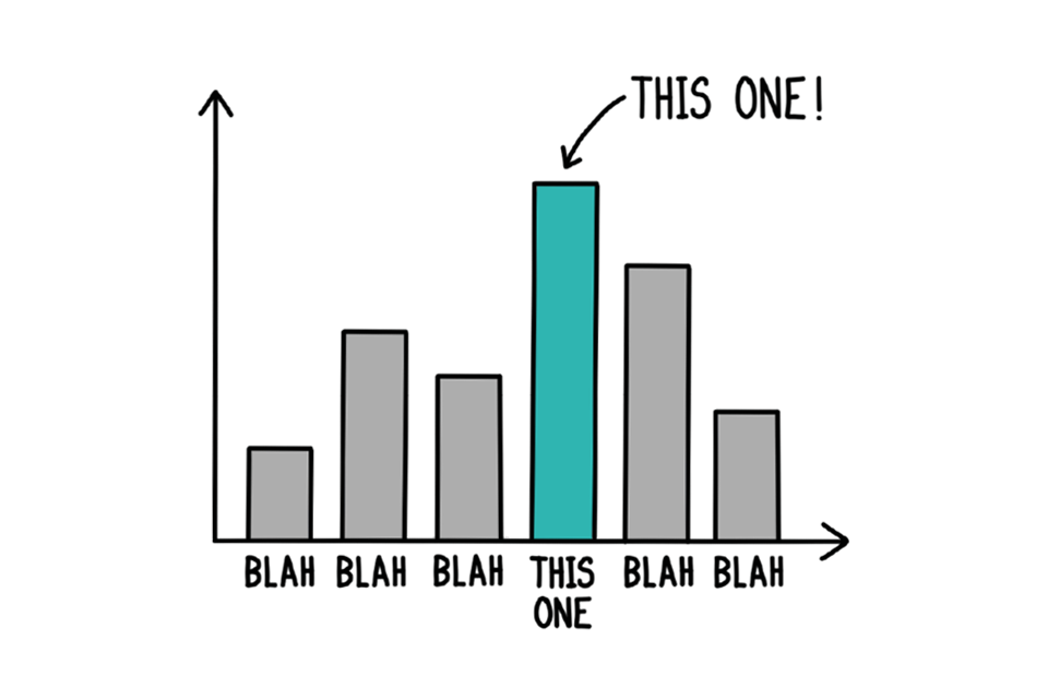
Example bar chart depicting five grey bars and one green bar.
Colour can also be changed dependent on what type of data you are working with. Categorical data, data that’s distinct from one another for example different types of biscuit, lend well to using a distinct colour for each category. A sequential colour palette (colours that transition from one to another) can be used when data is more continuous, for example population size across a country; the bigger the number the deeper the shade of the same colour. Divergent colouring can be used to show positive and negative changes from 0, with one colour getting deeper as it gets more negative whilst another colour gets deeper as it gets more positive.
Working memory
Attention limitations
People have limited attention when asked to do multiple activities at once. Where there are too many things at play, we get sensory overload and it is much harder to focus on the task at hand.
Take a look at the grids below to test how your visual memory works. Each grid contains a square with a unique colour that is not found elsewhere on the same grid. How quickly can you spot the unique colour for each one?
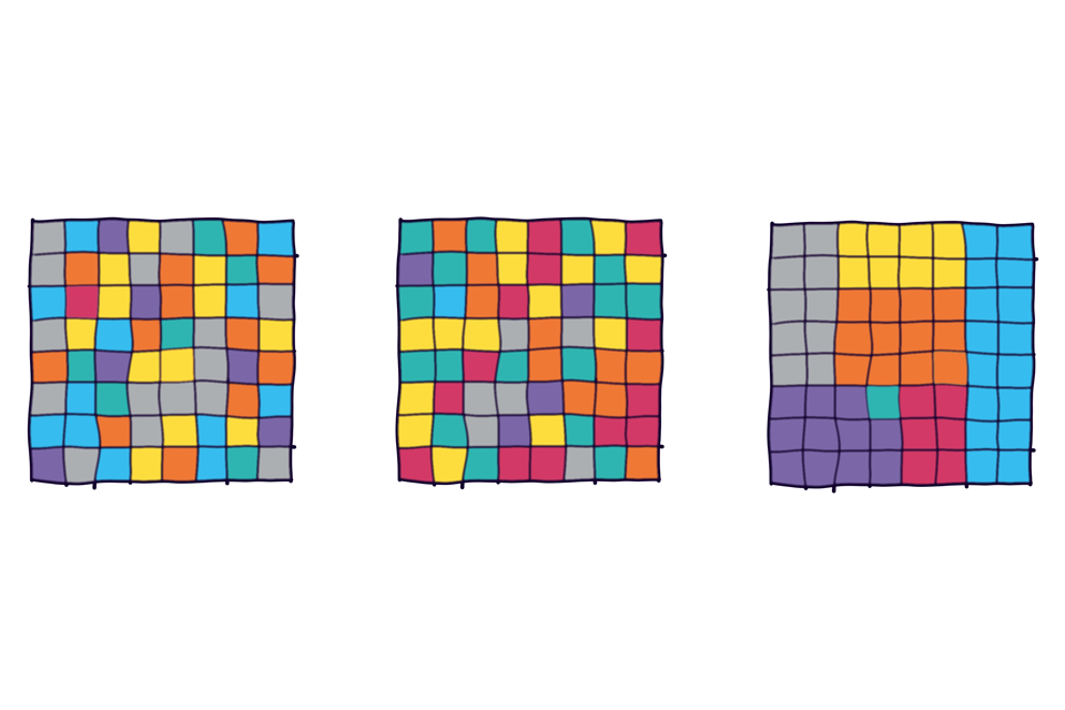
Three multi-coloured grids where only one has its colours organised into groups.
Three grids of mixed colours, each with one ‘unique’ colour that is found only on one square.
Some guiding principles
Psychologists have developed some guiding principles aimed at understanding how people perceive the world. We have collated, simplified and listed these below:
1) Law of simplicity
People will perceive and interpret ambiguous or complex images as the simplest form possible. This is because the brain is lazy, and doing this requires the least cognitive effort.
2) Figure-ground
When seeing an image, we usually focus on either the background or the foreground. There are many popular uses of this in modern day art, for example an image that in a white background shows two vases, but in the black foreground is a woman’s face. This logic is particularly useful when choosing backgrounds and foregrounds to help elevate a visual.
3) Similarity
When we see a group of similar objects, we tend to automatically group them together. Similarities can be in the form of visual properties such as size, colour, texture, dimension, shape or orientation. Similarity can be used in many graphs, for example we can group all biscuits that are circular and all those that are square by using their actual shapes!
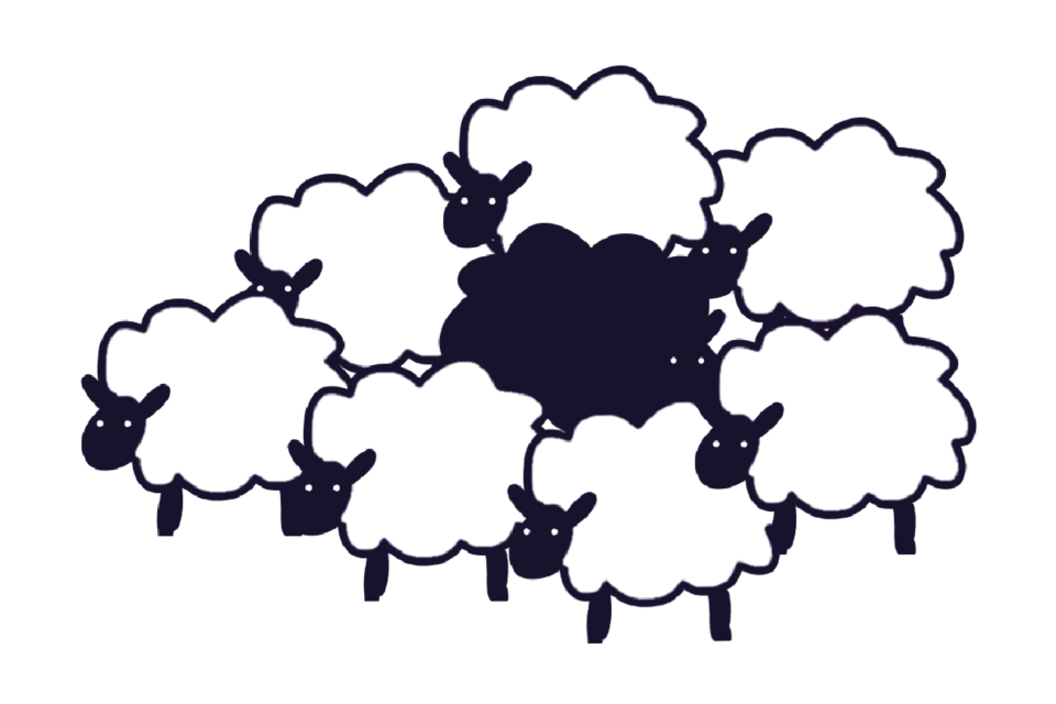
A flock of white sheep with a black sheep in the middle.
4) Proximity
We tend to group objects when they are close to each other, for example grouping biscuits by brand.
5) Closure
The brain can fill in gaps and create connections so we perceive a whole picture rather than lots of fragmented lines.
6) Organisation
Organisation has 3 key points:
-
Focal Point: Those objects that are different from the surrounding elements are more likely to stand out. This is particularly useful when you want a visualisation to land a key takeaway message.
-
Common Fate: Objects or elements that are moving in the same direction are also perceived as more related than those moving in a different direction or that are stationary.
-
Common Regions: Similar to proximity, we also identify objects to be related when they are in the same common regions. This is most commonly used when linking the headline, body of text and images in one area to help tell the story.
7) Continuity
Elements arranged in a line or a curve seem to be more related than those that are not. Something to consider when creating line graphs with multiple lines.
8) Symmetry
Another way in which people simplify complex images is via symmetry. Where something is symmetrical, we are more likely to perceive them as related.
Accessibility
In order to make data visualisation for everyone, we should try to make visualisations accessible and inclusive for as many people as possible. Accessibility covers a wide spectrum, and means we need to think carefully about the elements that make up a visualisation. It is very hard (or near on impossible) to cater to all, however there are some things we can do to improve the experience as much as we can. Below are a few things to think about when making visualisations as accessible as possible.
Use considerate colours
One of the easiest things to do is to carefully consider your colour choices. This can include avoiding colours that would look too similar to colour blind users (or anyone else for that matter!), adding whitespace space to graphs to split up colours and segments that are similar, and avoiding colours that contrast with the background. There are many tools available online that can help understand whether a visualisation has an accessible colour scheme or not. Some tools can even put a filter over the visualisation to show what it would look like to someone with a particular colour deficiency.
Add labels and annotations
Another way to make visualisations more accessible is to add labels and annotations. These not only help those who use assistive technologies like screen readers to understand what is displayed on a visualisation, but can also help the reader to unpack what the visualisation is really telling them. Using the title to briefly summarise what the visualisation shows and adding a more descriptive alternative text summary beneath a visualisation are two examples of best practice. It may also be useful to add labels to any data on the visualisation to highlight key points and help colour deficient users differentiate between data points instead of relying on the legend.
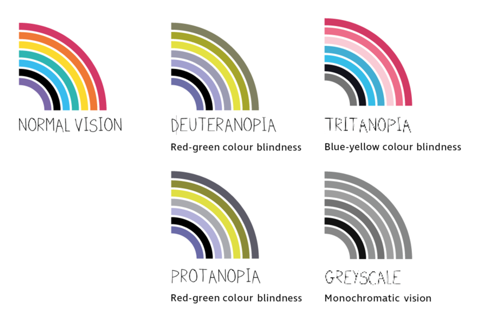
Five rainbows representing five spectrums related to colour perception.
Avoid complex tools
When creating interactive visualisations, it may be tempting to use lots of fancy tools that allow the user to interact with and manipulate the visualisation. Whilst interactivity can be useful and exciting, simplicity is key to keeping things more accessible. Avoiding things like sliders and replacing them with dropdown boxes can make the interactive elements more accessible to users with assistive technologies and easier to navigate using keyboard keys. Also, try to label any outputs instead of using tooltips or hovers-over a visualisation as these are difficult to use with assistive technologies.
Follow guidelines
Above are just a few examples of how to make a visualisation more accessible, and more guidance about how to best adapt your visualisation can be found online and in the community. Various organisations also have their own accessibility guidelines, including GOV.UK and the World Wide Web Consortium (W3C) which can be found online.
Visualisation options
When you know the story you want to tell, how do you get ideas for how to visualise it?
Resources for inspiration
There are many excellent resources online that show you different ways to present different types of data. Try searching for ‘graph gallery’ or ‘visualisation guide’ using your favourite search engine to get some ideas.
You can also get ideas for styles of visualisation from the news or online blogs, and even just lots of general information simply by searching online.
As well as getting ideas from online resources, there’s nothing wrong with brainstorming and coming up with ideas yourself. When you want to come up with ideas, we find it’s best to take the time to get away from your screen, have a cup of tea (and a biscuit), walk the dog, chat with someone or ‘sleep on it’. Some people even have their best ideas in the bath!
Conclusion
We hope you found this little book helpful.
Data Science is increasingly important to the way businesses operate and understanding the value that data can bring through careful analysis. It is therefore important to recognise that communicating the outcomes of such analyses is also very important – it’s not great to spend a whole heap of time on complex analysis if the outcomes are presented in a difficult to understand or confusing manner.
Visualisations are a great way to quickly present significant facts drawn from data, but as you’ve seen they can be a blessing and a curse – you did read the book didn’t you?
We hope therefore that this Biscuit Book has helped you to understand some of the most common ways that data is visualised so you may better understand what is being presented and become aware of the questions you should ask yourself about the way the visualisation has been constructed. Most importantly, ask yourself – is it doing what it says it is?
Happy viewing!