Research and analysis

Global supply chains: a foresight report on risk and resilience: annex B – agent-based modelling approach and scenario metrics

Updated 24 September 2026

1. Agent-based modelling approach

This section describes the agent-based modelling (ABM) approach that was used to support the analysis presented in Global supply chains: a foresight report on risk and resilience. A network modelling framework was used to explore how disruption can propagate through complex global supply networks and affect wider economic systems, helping to identify the structural features associated with supply chain vulnerability and resilience. The purpose of this section is to provide additional detail on the methods and assumptions underpinning the report’s findings. It outlines the rationale for using a network-based approach, the treatment of firms and supply relationships within the model, the assumptions required to represent complex production systems, and the limitations that should be considered when interpreting the results.

The purpose of the model was not to predict the exact outcome of future disruptions. Instead, it was used as a structured approach for exploring how different shocks may propagate through interconnected supply networks, identifying potential vulnerabilities and assessing how resilience varies across firms, countries and disruption scenarios.

1.1 Systemic risk in global supply chains

Global supply chains are not simple linear chains of production. Instead, they operate as complex networks in which firms are connected through multiple layers of upstream and downstream relationships. A disruption affecting one firm or country can therefore spread beyond the original point of impact through dependencies between suppliers and customers.

Systemic risk in multi-tier global supply chains refers to the risk that a localised shock propagates through interconnected supply networks and generates wider disruption. The consequences of a shock are therefore determined not only by the direct exposure of firms or countries, but also by their position within the wider production network.

These propagation dynamics operate in both directions. Downstream effects occur when disrupted firms are unable to supply their customers, reducing the availability of inputs for subsequent stages of production. Upstream effects occur when affected firms reduce their demand for inputs, lowering orders to suppliers and creating additional impacts further back through the network.

The scale of disruption therefore depends on network structure, including the number and importance of connections between firms, the concentration of supply relationships, and the presence of critical bottlenecks. As a result, an initial shock can generate disproportionately large effects through network-based transmission mechanisms.

Empirical and modelling studies demonstrate that these indirect effects can be significant and persistent. Inoue and Todo (2019) show that firm-level disruptions can propagate through supplier-customer relationships, causing losses that extend beyond directly affected firms. Similarly, Diem and others (2022) show that systemic importance is unevenly distributed across firms and is determined not only by firm size, but also by network position and production dependencies.

Understanding systemic risk therefore requires analysis of the wider network of relationships through which shocks propagate, rather than focusing only on direct trade exposure.

Conventional measures of direct trade exposure, such as import shares or supplier concentration, capture immediate, bilateral relationships but overlook the broader network structure. They therefore miss indirect dependencies, feedback effects and bottlenecks that can amplify disruption across tiers of production.

Linear or single-tier perspectives are similarly limited because they do not capture the non-linear dynamics of interconnected networks. They can understate the risks created by bottlenecks, low substitutability and multi-tier interdependencies.

Assessing systemic risk provides a fuller and more robust understanding of supply chain vulnerability by capturing both direct and indirect channels of impact, including non-linear propagation effects that conventional approaches may overlook.

1.2 Rationale for using network-based analysis and agent-based modelling 

Supply chain resilience depends on understanding connections between firms, not only measuring individual exposures.

Supply chain vulnerability is often assessed using concentration measures, such as the Herfindahl-Hirschman Indices (HHI), which can identify potential dependencies on a small number of suppliers or countries. These measures are valuable for identifying direct concentration risks, such as reliance on a single source of imports.

However, these measures are not sufficient for understanding systemic risk because they only capture direct exposures. They do not account for indirect vulnerabilities embedded within global supply chains, as described above. Therefore, at a minimum, concentration measures should be complemented by network and centrality metrics to provide a more accurate assessment of supply chain vulnerability.

Network-based measures provide additional insight by considering the position of firms and countries within the wider supply structure. Centrality measures capture different aspects of network importance:

• degree centrality captures the number of direct connections a firm or country has, making it a useful proxy for immediate exposure to network flows
• betweenness centrality identifies firms or countries that act as important intermediaries by connecting otherwise separate parts of the network, highlighting potential bottlenecks
• eigenvector centrality places greater weight on connections to other important nodes, providing an indication of where influence and risk may propagate through highly or importantly connected parts of the network

As noted by Ledwoch, Yasarcan and Brintrup (2018), the use of centrality measures in supply chain analysis remains relatively limited. They also state that each measure should be treated as a partial indicator rather than a complete measure of systemic importance. Together however, these metrics can provide transparent and tractable diagnostics of network structure. However, because they are largely static, they do not capture how disruptions propagate dynamically across multiple tiers. They may therefore miss indirect dependencies, feedback effects and non-linear amplification. They are therefore most useful when combined with approaches that explicitly simulate disruption pathways.

Agent-based modelling complements network analysis by modelling how individual firms interact and how these interactions generate system-wide outcomes.

To examine the impact of shocks and to estimate the resilience of the inter-firm supply network, we use an ABM to compute an Economic Systemic Risk Index (ESRI) for each firm and country. This approach explicitly represents firm-level heterogeneity, multi-tier supplier relationships and the propagation of shocks through cascading upstream and downstream effects.

Firm-level modelling

Firm-level modelling is critical because supply networks are not made up of identical firms. Companies operating in the same sector or country can have very different roles within production networks depending on their suppliers, customers, products and position within the wider system. These differences influence whether a disruption remains localised or develops into a wider systemic shock.

Aggregated approaches that represent firms only at the sector or country level can therefore hide important features of the underlying production network. By treating firms as equivalent, these approaches may overlook critical suppliers, highly connected firms, or concentrated dependencies that determine how shocks propagate.

Diem and others (2024) demonstrate the importance of maintaining firm-level detail by comparing firm-level production networks with aggregated sector-level representations. They show that aggregation can underestimate the economic impact of disruptions because it removes heterogeneity in network structure. In particular, aggregation obscures differences in supplier concentration, connectivity and the position of individual firms within production networks.

For example, 2 firms operating in the same industry may have very different levels of systemic importance. One firm may have several alternative suppliers and customers, allowing it to absorb disruption relatively easily. Another may provide a critical input to many downstream firms or rely on a small number of specialised suppliers. Treating both firms as equivalent at the sector level can therefore hide important vulnerabilities.

Firm-level relationships are also essential for understanding how shocks propagate through supply networks.

Inoue and Todo (2019) demonstrate that economic disruptions spread through the specific connections between firms rather than simply affecting entire industries. Their firm-level model of the Japanese economy represents firms as connected through supplier–customer relationships and simulates how disruptions propagate through these links.

Their findings show that the effects of a shock extend beyond directly affected firms. When a disrupted firm cannot provide inputs to its customers, those customers may reduce their own production, creating further impacts across the network. These cascading effects emerge from many individual firm-level interactions, demonstrating why aggregated approaches cannot fully capture the pathways through which disruption spreads.

The importance of individual firms within these networks is further highlighted by Diem and others (2022). They show that systemic risk is highly unevenly distributed across firms, with a relatively small number of firms accounting for a disproportionate share of potential economic impacts. Importantly, systemic importance is not determined solely by firm size. Firms can become systemically important because of their position within the network, the uniqueness of their products, or their role as suppliers of critical inputs.

Together, this evidence supports modelling supply networks at the firm level and explicitly representing firms as heterogeneous agents. By capturing differences in firm characteristics and network position, ABM provides a more realistic representation of how shocks originate, propagate and amplify through complex production systems.

1.3 Modelling framework description

Building on the rationale outlined above, we now describe the ABM framework used to examine the impacts of disruption and estimate the vulnerabilities and resilience of supply networks.

An ABM represents a system as a collection of individual actors, known as agents, and models how their interactions generate system-wide outcomes. In this context, firms are the agents. Each firm has its own production characteristics, supplier relationships and position within the supply network. The model follows the ABM framework developed by Diem and others (2022, 2024), which links firms through observed input-output relationships using firm-level transaction data.

Figure 1: Illustrative representation of a firm within the supply network model, created by GO-Science

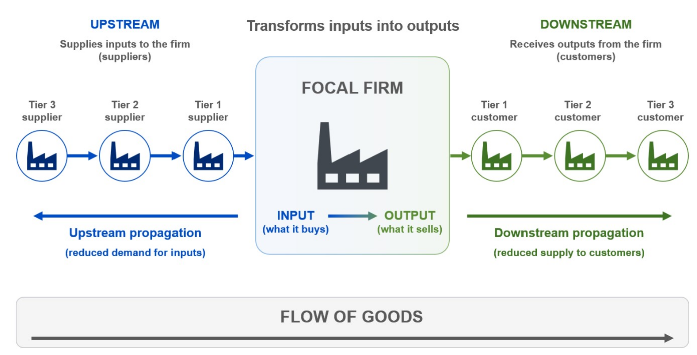
Alt text: Figure 1 shows a supply network model with a focal firm between upstream suppliers and downstream customers, with goods flowing from suppliers through the firm to customers.

Each firm is linked to a set of input and output products as specified by the underlying product-level data. Within the ABM, individual firms interact through a supply network and transform input products into output products, subject to their internal production capacity, the availability of required inputs and the level of demand for their outputs. This allows the model to capture firm-level heterogeneity in production roles and network position, rather than treating all firms within a sector or country as identical.

Production constraints

The model represents firm production using a generalised Leontief production assumption. A Leontief production function assumes that production requires a fixed combination of essential inputs. Therefore, output is constrained by the least available required input: a shortage of one critical input cannot be compensated for by having additional quantities of other inputs. In practical terms, firms are assumed to require all essential inputs to produce output.

While firms cannot replace unavailable inputs with alternative inputs within the model, if available, they can adapt by finding alternative suppliers for products whose production by their previous supplier has been disrupted. This simplifies production decisions and allows disruption pathways to be traced clearly through the supply network.

The Leontief assumption therefore represents a conservative modelling choice. By limiting firms’ ability to substitute inputs, the model may generate stronger cascading effects than would occur if firms were able to adapt fully. However, this reduces the risk of understating systemic vulnerability and provides a cautious assessment of resilience under severe disruption scenarios.

Supplier replaceability

The model also includes a system-level notion of supplier replaceability, following Diem and others (2022). The impact of disrupting a supplier depends partly on how easily that supplier can be replaced within the wider market for a product.

A disruption affecting a supplier that represents a large share of available supply could generate greater cascading effects than a disruption affecting a supplier with many comparable alternatives. However, there may be many comparable substitutes, minimising cascading effects. Replaceability depends not only on a supplier’s share of available supply, but also on the availability of suitable substitutes within the wider market for that product. This allows the model to distinguish between vulnerabilities caused by concentrated supply relationships and those occurring in more diversified networks.

Treatment of links

Links in the model represent trading relationships between firms, connecting suppliers with customers across multiple tiers of production. These relationships form the structure through which disruptions propagate.

Unlike approaches that only consider direct bilateral trade relationships, links in the model capture indirect dependencies between firms. For example, a disruption affecting one firm may influence other firms several stages away through their supplier and customer relationships. The structure of these connections, including the position of firms within the network and their dependence on particular suppliers or customers, influences whether a shock remains localised or generates wider systemic impacts.

Treatment of shocks

Production shocks are modelled as exogenous reductions in firm-level production capacity. Although shocks are introduced at the firm level, the model can represent larger-scale events. For example, it can model regional or national disruptions. It does this by reducing capacity across affected firms. It can also vary impacts according to geographical distance from the shock origin.

For simplicity, where firms produce multiple outputs, the same proportional reduction in capacity is applied across all products. This provides consistency across scenarios but does not capture cases where specific product lines or facilities might experience different levels of disruption.

In our exploratory application of the model, affected firms or countries are assumed to lose all production capacity following a shock. This represents an extreme disruption scenario rather than a prediction of the most likely outcome of a future event. The shocks used in our analytical framework are neither likely nor aspirational, and no assumptions are made about their accuracy as forecasts of future events. Instead, they are designed to help examine how supply networks could respond under disruption at all points of the supply network. This enables the identification of specific firms, countries, or geographical areas that may be particularly exposed to disruption and therefore warrant further policy attention.

Once the shock occurs, it propagates through the network in 2 directions. Downstream propagation occurs when affected firms supply fewer inputs to their customers, limiting those customers’ own production. Upstream propagation occurs when affected firms reduce their demand for inputs, lowering orders to their suppliers.

The model compares a baseline steady state with a post-shock equilibrium. Starting from the pre-shock supply network, a disruption is introduced and firms iteratively update their realised production in response to changes in input availability, demand conditions, and production capacity. The propagation process continues until the network stabilises at a new equilibrium. The difference between the baseline and post-shock equilibrium is then used to assess the scale of systemic disruption and the resilience of the supply network.

1.4 Data source

The supply chain network is mapped using firm and transaction-level data from the UK government Global Supply Chain Intelligence Programme (GSCIP), which provides tools and data for supply chain mapping. The model uses the underlying commercial dataset rather than the enhanced government datasets available through GSCIP. The dataset combines international trade documentation (including bills of lading and logistics records) with company information such as firm location and sector classification.

GSCIP enables the identification of firm-to-firm product flows and the construction of a multi-layer supply network, where each product category (defined using Harmonized System 6-digit product codes, HS6) is represented as a separate network layer. This level of granularity is particularly valuable for systemic risk analysis because it allows the model to capture dependencies between individual firms and products rather than relying only on country- or sector-level trade statistics.

We use a 5-year time period, from 1 January 2020 to 31 December 2024, to map supply chains from the data. The most recent year is excluded because of delays in data reporting and updates. A 5-year time period is preferred to a shorter 2-year time period because it provides a more complete view of supply relationships that may only appear intermittently in transaction data.

This is particularly important for supply chain tiers such as raw materials, where firms may batch orders to reduce transport costs. These transactions can be infrequent but large, meaning shorter observation periods are more likely to miss important high-volume links and produce a less accurate representation of the network.

A longer time period also helps capture contingency relationships, such as multi-sourcing and backup suppliers. These are common supply chain risk management practices (Tang, 2006), but backup suppliers may only be used during periods of shortage or delay because they are often more costly than regular suppliers. Including the COVID-19 period therefore helps reveal some of these backup connections, which are relevant for modelling resilience under stress.

Using a longer period also has drawbacks. It can include some trade links that are no longer active, and the 2020 to 2024 period overlaps with the COVID-19 pandemic, when supply chains were unusually disrupted. We mitigate the risk of outdated links by constructing a weighted aggregate network, in which older connections receive lower weights.

The COVID-19 period affects the data in 2 ways. First, it introduces temporary disruption, including delivery delays and distorted transaction volumes. These effects are less likely to change the underlying firm-to-firm network structure, particularly because delayed products are eventually delivered and links are weighted by transaction volume. Second, the pandemic led to more lasting changes in sourcing patterns, including diversification and rerouting of supply chains, for example through ‘China plus one’ strategies (Niu and others, 2025). These structural changes are relevant to the analysis and should be reflected in the network.

Given that modelling network adaptation is beyond the scope of this project, we consider it preferable to use data that captures how firms adjusted during a large-scale shock such as COVID-19. The proportional weighting of trade links also means that low-weight or peripheral connections have limited influence on overall network dynamics.

Why GSCIP was selected

GSCIP was selected because the analysis requires firm-level, product-level and internationally connected supply chain data.

Alternative datasets provide useful but different information. For example, databases such as FactSet and Bloomberg identify buyer–supplier relationships but generally do not provide the same level of product-level detail. The United Nations (UN) Comtrade provides extensive international trade information but is reported at the national level and therefore cannot capture firm-level supply relationships.

Some national datasets provide more detailed product-level information, but these are generally limited to individual countries and cannot represent internationally connected supply networks.

The 2 most suitable international firm-to-firm product-flow datasets considered were GSCIP and Standard and Poor’s (S&P) Panjiva. Both provide information derived from trade and logistics records, although both have stronger coverage of international flows than intra-national supply relationships.

GSCIP was selected because it is already widely used across government, making the approach more accessible for future analytical applications. It also includes extensive preprocessing by data providers and integrates additional information on companies, financial characteristics and risk indicators. The dataset was selected following cross-government appraisal as the most suitable and cost-effective option for the objectives of this analysis.

Data limitations and interpretation

Like all large-scale supply chain datasets, GSCIP has limitations in coverage and completeness. These limitations are important when interpreting highly granular results, particularly rankings of individual firms or countries.

Company matching within GSCIP is probabilistic. Whilst extensive effort has been made to identify and link records relating to the same firm, some entities may not be matched correctly, some relevant entities may be absent from the dataset, and the same organisation may appear under multiple identifiers. As a result, trade activity associated with a single firm may be fragmented across several entities within the model. This can lead to an understatement of a firm’s apparent scale, connectivity, or influence within the production network.

One limitation is that capturing intra-national supply relationships is not a capability offered by GSCIP, so while some domestic transactions can creep in, these are much less well captured than cross-border flows, for which GSCIP is explicitly designed. Cross-border movements of goods generate extensive data through mandatory import and export declarations, customs processes, and border controls, providing the evidence base for supply chain mapping offered by GSCIP. Equivalent reporting requirements generally do not exist for the movement of goods within national borders, meaning domestic supply relationships are inherently less visible. Coverage also differs across jurisdictions, with some countries having more comprehensive reporting systems than others. As a result, certain countries may appear more prominently within the observed network, while countries with weaker data coverage may appear less connected or systemically important than they are in reality. Similar challenges exist for some raw material supply chains, where extraction, processing, and intermediate production stages may be difficult to observe through trade and logistics records alone.

The nature of logistics data can also introduce biases into the observed network structure. Countries that function as major transhipment or distribution hubs may be over-represented because large volumes of goods pass through them before reaching their final destination. This can make some locations or firms appear more central within the network than their underlying role in production would suggest. Conversely, firms or regions with less complete data coverage may appear less influential despite having significant real-world importance.

To address these challenges, the modelling framework incorporates reconstruction and imputation methods to estimate missing relationships and financial values. The extent of imputation varies across products and jurisdictions depending on data availability.

In addition, financial values used may be affected by incomplete reporting. These factors introduce uncertainty into the precise measurement of firm- and country-level importance within the network.

These limitations affect how results should be interpreted. The model is most reliable for identifying broad patterns of vulnerability and understanding how shocks propagate through network structures. More caution is required when interpreting the precise ranking of individual firms, regions or countries. Where specific entities are identified as highly systemically important, results should be considered alongside expert judgement and contextual knowledge.

The findings should therefore be interpreted as insights from the observed and reconstructed network, rather than as a complete measurement of all global production relationships.

1.5 Model assumptions

The ABM relies on a set of simplifying assumptions about firm behaviour, production processes and shock propagation. These assumptions are necessary to make the model tractable and interpretable, but they also shape how the results should be understood.

Leontief production assumption

As considered by Ledwoch, Yasarcan, and Brintrup (2018), Inoue and Todo (2019), and Diem and others (2022), firms are represented by generalised Leontief production functions to link inputs and outputs of individual firms.

A Leontief production function assumes that production requires a fixed combination of essential inputs. Consequently, output is constrained by the least available required input, meaning that a shortage of any critical input limits production regardless of the availability of other inputs.

Under this assumption, inputs are treated as complements rather than substitutes, meaning that firms cannot replace unavailable inputs with alternatives. Non-essential goods and services that may improve productivity are also excluded. This provides a simplified representation of production processes and supply chain dependencies, allowing disruption pathways to be traced clearly through the network. In reality, firms may substitute suppliers, redesign products, modify production processes or adjust operations following disruption.

By assuming that production is limited by the availability of essential inputs, the model tends to generate stronger cascading effects than approaches that allow input substitution. This represents a conservative modelling choice that reduces the risk of understating potential supply chain vulnerabilities and systemic impacts, although it may overstate the extent of disruption where firms could adapt successfully.

Fixed product mix and supplier relationships

Although we allow for firms in the ABM to produce more than one output, their product mix is assumed to remain fixed during the disruption. In practice, this means no supplier switching or production adaptation is modelled.

This simplifies the representation of firm behaviour and ensures that changes in output are driven by network structure, input availability and demand conditions rather than strategic decisions. Although one could model the firm’s product mix and supplier switching decisions, using a search and matching approach similar to Zhao, Zuo, and Blackhurst (2019), it increases the computation time substantially. Hence, we use a simpler model and do not capture the impact of firm-level product mix change and supplier switching.

In practice, firms may respond to disruption by identifying alternative suppliers or reallocating production. However, these responses are often costly and constrained by technical compatibility, contracts, regulatory requirements and the time needed to establish new relationships. The implication is that the model represents vulnerability in the existing supply network rather than the full adaptive capacity of firms.

Fixed network structure

The set of firms in the network is assumed to remain fixed during the simulation. While network structure may evolve through rewiring during the projection stage, the model does not explicitly represent firm entry, exit, mergers, acquisitions, or other forms of long-term market restructuring. Where a firm is assumed to leave the network, its role is treated as being replaced by other firms occupying a similar network position rather than removed from the system entirely.

This limits the ability to analyse how industries may transform over long periods following disruption. However, it is unlikely to materially affect the model’s primary purpose: understanding how shocks propagate through existing supply relationships.

Shock representation

Shocks are represented as proportional reductions in a firm’s production capacity, as a baseline entailing complete reduction of production. Where a firm produces more than one output, the same capacity reduction is applied across all its outputs. This provides a consistent way to model firm, region, country or bloc-level shocks, without requiring additional assumptions about which individual product lines would be affected first.

In reality, shocks may affect different activities within a firm unevenly, with some products or facilities experiencing greater disruption than others. Applying a uniform capacity reduction therefore simplifies the nature of real-world disruptions and may not capture all sources of operational complexity. However, this assumption enables consistent comparison across scenarios and ensures that differences in model outcomes are driven primarily by network structure and shock characteristics rather than by product-specific assumptions. The results should therefore be interpreted as illustrating how disruptions propagate through supply networks rather than predicting the exact impacts on individual product lines.

1.6 Main exclusions

The model is designed to identify systemic vulnerabilities, not to reproduce all aspects of real-world supply chain behaviour.

To remain computationally tractable and focused on shock propagation, the model excludes several processes that influence how firms respond to disruption in practice. These exclusions mean that the results should not be interpreted as precise forecasts of future outcomes or predictions of how individual firms would behave following a real-world event.

Instead, the model provides a structured stress test of supply chain resilience. It illustrates how vulnerabilities may emerge and propagate through existing supply networks under different disruption scenarios.

Firm adaptation and behavioural response

The model does not predict future demand, trade flows, production levels or the likelihood of specific disruption events. It also does not capture behavioural adaptation after a shock.

Consistent with the Leontief-type production assumption, firms are not assumed to substitute inputs, switch suppliers, change product mix, redesign production processes or adjust strategically in response to disruption. This simplifies the representation of firm behaviour and allows the model to isolate how shocks propagate through existing supply chain structures.

However, it represents a conservative modelling choice, as firms may be able to partially absorb disruptions in practice through alternative sourcing, inventory use, or operational adjustments. As a result, the model may overstate the extent of cascading effects by limiting the adaptive capacity of firms.

Inventories and timing effects

The model does not explicitly represent inventories, buffer stocks or stock drawdown.

In practice, firms may temporarily absorb supply disruptions by using existing inventories or adjusting stock levels. Because these mechanisms are not represented, the model may show disruption occurring more quickly than it would in reality.

The model also excludes transport delays and production lead times. As a result, it captures the eventual scale and distribution of disruption through the network rather than the precise timing of impacts.

This means the results should be interpreted as showing where vulnerabilities exist and how disruptions may propagate, rather than predicting when impacts would materialise.

Logistics networks and supply chain completeness

The model does not fully represent the physical logistics network, including ports, shipping routes, transport capacity or route-specific bottlenecks.

Similarly, the underlying supply network should not be interpreted as a complete map of all global production relationships. Coverage depends on the available transaction data and may be weaker for some countries, sectors, raw material supply chains and intra-national relationships.

These limitations mean that individual firms or locations may appear more or less systemically important depending partly on data visibility. However, the model remains valuable for identifying broad patterns of dependency, comparing alternative scenarios and understanding how shocks propagate through observed supply structures.

1.7 Model output: Economic Systemic Risk Index

The main output from the ABM is the ESRI, which is calculated for each firm and country in the supply network.

Following Diem and others (2022), ESRI measures the reduction in production output caused by the complete disruption of a given firm, region or country, relative to the baseline. It is designed to move beyond direct exposure metrics by capturing indirect, multi-tier dependencies and identifying entities that are systemically important, even where they appear less significant in direct trade statistics. A firm may have a modest direct trade role but still have a high ESRI if it sits at a bottleneck in the network or is part of a critical dependency. This metric helps identify firms, regions and countries that are systemically important for selected case study products. It can compare the relative vulnerability of supply networks and can also help explain how shocks cascade through multi-tier supply structures.

The model reports 2 versions of the index. Global ESRI measures the percentage of total output at risk across all firms in the supply network, while UK ESRI measures the percentage of output at risk across UK-based firms only. This distinction allows the analysis to separate impacts on the global network from those that are most directly relevant to UK resilience.

The outputs are intended to support foresight and resilience analysis rather than point prediction. They should therefore be interpreted as structured stress tests of systemic vulnerability, not as precise forecasts of future trade flows, production losses or firm behaviour.

The results should also not be read as complete measurements of all real-world supply relationships, evidence that a given disruption will occur, or a full representation of firm adaptation such as supplier switching, inventory use or strategic changes in product mix. Instead, they are most useful for comparing relative risk across firms, regions, countries and scenarios.

2. Headline metrics: methodology and interpretation

This section sets out the methodological approach used to develop, select, and validate the metrics that provide a quantitative sense of difference for the Future of Global Supply Chains scenarios. Metric identification and final selection of the 6 headline metrics were led by GO-Science, while the metric projection approach, supporting analysis, and scenario-specific projections were developed by Forgefront, an external supplier, working closely with GO-Science and subject matter experts.

2.1 Purpose and aims

The metrics were developed to collectively illustrate the state of global supply chains in 2040 against the 4 future scenarios created for this foresight project, spanning both climate and geopolitical uncertainties. Their purpose is to provide a transparent, evidence-based means of comparing and visualising differences between scenarios. They help illustrate how trade, climate, and geopolitical factors could evolve under different future conditions.

The metrics are informed by quantitative data and expert input, but they are not forecasts or predictions. Instead, they are illustrative tools, grounded in evidence and expert judgement, designed to support scenario comparison and policy thinking. The 6 headline metrics and the illustrative estimates used to represent conditions within each scenario were selected by GO-Science using evidence from across the project, including underlying analysis undertaken by ForgeFront.

We thank ForgeFront for their contribution to the wider analytical process that informed the development, testing, and refinement of the metrics presented in the report.

2.2 Methodological approach

The methodology for developing the metrics followed 2 distinctive phases: An initial longlist of metrics was developed in-house by GO-Science (step 1 below), while Forgefront developed the projection methodology, supporting analysis, and scenario-specific projections (steps 2 – 4), with a final step (5) providing a sense of confidence completed by GO-Science.

Step 1: initial in-house metric development

GO-Science developed an initial longlist of candidate metrics through a structured, in-house process, including workshops and expert engagement across government. Candidate metrics were reviewed, consolidated, and prioritised based on their relevance to the project’s critical uncertainties and their suitability for scenario quantification. This produced a prioritised shortlist of metrics for further development and testing.

Step 2: desk research and data verification

The external supplier reviewed the candidate metrics and identified suitable data sources to support their measurement. Where necessary, metrics were adapted or refined to ensure robust coverage of the scenario uncertainties and the availability of suitable historical data.

Step 3: data extrapolation and scenario-specific projections

The external supplier first reviewed, cleaned, and standardised historical datasets to create consistent annual time series and an evidence base for projecting how each metric could evolve to 2040. Using this evidence base, they applied historical trend analysis and quantitative extrapolation to develop baseline projections for each metric in each scenario. Working closely with GO-Science, they then assessed how these projections might change under the conditions described in each of the 4 scenarios. Different metrics required different approaches depending on data availability, historical behaviour, and the availability of relevant historical analogues.

Step 4: expert verification and adjustment

To ensure the projections were robust and reflected the intended scenario characteristics, an expert panel was convened, comprising specialists from academia, industry, and the public sector with expertise in climate and geopolitics. Experts were invited to review and adjust the projected metric values, providing both quantitative input and qualitative feedback. Statistical analysis of expert responses was used to assess consensus and guide adjustments. Where sample sizes were low or confidence was limited, qualitative insights were used to refine projections. This process ensured that the final metrics were not only evidence-based but also subject to independent scrutiny and challenge.

Given the exploratory nature of the exercise and varying levels of confidence across the metrics, the resulting values are presented as rounded figures throughout the report to emphasise scenario comparison and avoid implying undue precision.

Step 5: confidence ratings and final selection

To ensure analytical rigour, GO-Science created simplified confidence ratings for each metric, combining the following factors:

• supplier confidence in attributing historical time ranges to each scenario-metric pairs rather than using the baseline in step 3
• number of experts contributing to verification in step 4
• degree of divergence between expert consensus and initial projections in step 4
• level of agreement among experts in step 4

Metrics were rated from high to low confidence. The final set of 6 headline metrics was selected based on their ability to represent the scenario uncertainties, illustrate differences between the scenarios, and provide sufficient confidence for quantitative comparison. To ensure balanced coverage across the scenario framework, 2 metrics were selected for each of the trade, climate and geopolitics dimensions. These were:

• trade generic: global trade intensity (high); UK trade integration (high)
• climate adaptation: climate shock exposure (medium-low); societal readiness for climate adaptation (medium-high)
• geopolitical fragmentation: global trade cooperation (high); alignment with trusted trade partners (medium-high)

Including one medium-low confidence metric was considered defensible, as the aim is illustrative comparison rather than precise forecasting.

2.3 Limitations and interpretation

While every effort was made to ensure methodological rigour and transparency, there are inherent limitations to this approach. Data availability and quality varied across metrics, and some projections relied on qualitative judgement where quantitative evidence was lacking. Expert participation, though diverse, was below the targeted sample size. Some metrics received fewer than 10 responses, making results indicative rather than definitive.

Most importantly, the metrics are not forecasts or predictions. They are scenario-specific illustrations, designed to support comparative analysis and strategic thinking, not to provide precise estimates for planning or investment.

2.4 Overview of headline metrics

The 6 headline metrics were selected to provide illustrative, evidence-informed indicators of how trade, climate adaptation and geopolitics could evolve across the 4 scenarios. For transparency, this section summarises the purpose of each metric, the data source used, and considerations for interpretation.

2.4.1 Metric 1: global trade intensity

Dataset	UN Comtrade
Organisation	UN Statistics Division
Coverage	1989 to 2023
Category	Trade generic
Confidence	High
How to read this metric	A higher value indicates greater levels of international trade.

This metric was selected as a high-confidence indicator of the overall scale of international trade and provides contextual information for the other metrics. It measures the total value of goods exports reported internationally and therefore acts as a broad indicator of global trade activity and supply chain integration. A higher value (measured by US dollar) indicates greater levels of international trade.

Data are drawn from UN Comtrade, which compiles internationally reported merchandise trade statistics from participating countries. The UN Comtrade Processing System integrates the processing and dissemination of all trade data by the reporting country, including:

• annual international merchandise trade statistics (IMTS)
• monthly IMTS and annual statistics in trade services (SITS)

The metric should be interpreted as an indicator of the overall direction and scale of global trade rather than a prediction of future export volumes.

2.4.2 Metric 2: UK trade integration

Dataset	UK total trade: all countries
Organisation	Office for National Statistics (ONS)
Coverage	1948 to 2024
Category	Trade generic
Confidence	High
How to read this metric	A higher value in pounds indicates the UK exports more goods and services to other countries.

This metric was selected as a trade generic metric because it captures the UK’s position and performance within global trade and supply chains, offering a measure of national economic engagement and resilience under different future conditions. The metric should be interpreted as an indicator of broad trade orientation rather than a measure of trade performance or desirability.

The data are drawn from the UK’s ONS, covering UK imports and exports. This value represents exports of goods and services. A higher value in pounds indicates the UK exports more goods and services to other countries.

UK Trade statistics compiled by ONS are measured monthly and quarterly through both imports and exports of goods and/or services. Data is supplied from over 30 feeder sources including a variety of administrative sources, the main one being HMRC.

2.4.3 Metric 3: climate shock exposure

Dataset	Our World in Data (OWID)
Organisation	Global Change Data Lab
Coverage	2000 to 2023
Category	Climate adaptation
Confidence	Medium low
How to read this metric	A higher number means climate disasters are becoming more frequent, signalling greater disruption and risk.

This metric was selected to provide an indication of the frequency and exposure of global supply chains to climate-related shocks. A higher value indicates a greater number of climate-related disruption events occurring in a given scenario and therefore a higher likelihood of damage to infrastructure, production, and trade networks. The metric is based on internationally reported climate-disaster data and should be interpreted as an indicator of exposure to climate-related disruption rather than a prediction of specific future events or losses.

This metric looks at the frequency of climate disasters. According to the Centre for Research on the Epidemiology of Disasters’ (CRED) Emergency Events Database (EM-DAT), climate disasters are deemed:

• as extreme weather and climate-related events, such as floods, droughts, storms and wildfires
• to cause significant disruption and overwhelm local capacity, necessitating a request for external assistance at the national or international level

They are unforeseen and often sudden events that cause significant damage, destruction, and human suffering.

This metric draws on data from OWID’s published visualisation of EM-DAT’s ‘Number of recorded natural disaster events’ dataset. This has been filtered according to EM-DAT’s ‘natural disaster category’ from the year 2000 onward, including only ‘drought’, ‘wildfire’, ‘glacial lake outburst flood’, ‘extreme temperature’, ‘fog’ and ‘extreme weather’, to reflect the definition above.

2.4.4 Metric 4: societal readiness for climate adaptation

Dataset	DESNZ Public Attitudes Tracker
Organisation	Department for Energy Security and Net Zero (DESNZ)
Coverage	2012 to 2025
Category	Climate adaptation
Confidence	Medium high
How to read this metric	A higher percentage indicates that more people are concerned about climate change.

This metric was selected as an environmental indicator of public awareness and societal readiness for climate action, which can influence both policy responses and the effectiveness of adaptation strategies, one of the main uncertainties in our scenarios. It should be interpreted as an indicator of public sentiment towards climate change as a policy issue rather than a direct measure of adaptation capability or policy effectiveness.

The metrics draws on data from the Public Attitudes Tracker, a triannual survey collecting data on public awareness, behaviours, and attitudes relating to the policy areas of the different departments that have managed it. These include:

• the Department for Energy Security and Net Zero (DESNZ, 2021 to present)
• the Department for Business, Energy and Industrial Strategy (BEIS, 2016 to 2021)
• the Department of Energy and Climate Change (DECC, 2012 to 2016)

The survey measures the percentage of adults in the UK concerned about climate change. A higher percentage indicates that more people are concerned about climate change, a lower number indicates that fewer people are concerned.

Methodologies changed as departments evolved but the questions remained the same. Our focus is on the climate concern question ‘How concerned, if at all, are you about climate change, sometimes referred to as ‘global warming’?’, to which respondents could reply ‘Very concerned’, ‘Fairly concerned’, ‘Not very concerned’, ‘Not at all concerned’, ‘Don’t know’. Responses were then aggregated into 2 buckets: ‘Net: Total concerned’ and ‘Net: Total not concerned’.

2.4.5 Metric 5: global trade cooperation

Dataset	Regional Trade Agreements Database
Organisation	World Trade Organization (WTO)
Coverage	1949 to 2024
Category	Geopolitical fragmentation
Confidence	High
How to read this metric	A higher number means more regional trade agreements exist, signalling greater trade cooperation and integration.

This metric was selected as a geopolitical indicator  of international trade cooperation and integration, combining elements of both trade and geopolitics that are highly relevant to supply chain resilience and fragmentation. It reflects the existence of formal agreements and should not be interpreted as a measure of their effectiveness, depth, or implementation.

Data are sourced from the WTO’s Regional Trade Agreements (RTA) Database, a comprehensive database of all RTAs notified to the General Agreement on Tariffs and Trade or WTO. RTAs are reciprocal preferential trade agreements between 2 or more parties. It tracks the number of RTAs, including both existing and newly established agreements. A higher value means more regional trade agreements are in place.

2.4.6 Metric 6: alignment with trusted trade partners

Dataset	Trade in goods and services: all countries, seasonally adjusted
Organisation	ONS
Coverage	1997 to 2024
Category	Geopolitical fragmentation
Confidence	Medium high
How to read this metric	Higher values indicate the UK is trading more with nearby countries as a share of its overall trade.

Dataset overview

This metric was chosen as a geopolitical indicator of geopolitical alignment in trade relationships, which in our scenarios often overlaps with trade bloc membership and signals a preference for trading with allies over more distant or less aligned countries. Although the underlying measure uses UK-EU trade, the metric is not intended to represent trade with the EU specifically. Instead, it serves as an indicator of trade patterns shaped by geopolitical alignment, such as those seen in Scenarios C and D. Higher values indicate a greater proportion of UK trade taking place within closely integrated trading relationships.

This metric draws on data from HMRC’s Trade in goods statistics (TIGS) from the ONS. This covers the UK’s international trade in goods at a disaggregated country and product level. It measures the share of UK trade with the EU and includes both imports (UK trade imports from the EU) and exports (UK trade exports to the EU). A higher value indicates more trade with the EU as a share of overall UK trade, a lower value indicates less trade with the EU as a share of overall UK trade.

3. References

Diem, C, Borsos, A, Reisch, T and Kertész, J. ‘Quantifying firm-level economic systemic risk from nation-wide supply networks’ 2022: Scientific Reports, 12, 7719.

Diem, C, Borsos, A, Reisch, T, Kertész, J and Thurner, S. ‘Estimating the loss of economic predictability from aggregating firm-level production networks’ 2024: PNAS Nexus, 3(3), page 064.

Inoue, H and Todo, Y. ‘Firm-level propagation of shocks through supply-chain networks’ 2019: Nature Sustainability, 2, pages 841 to 847.

Ledwoch, A, Yasarcan, H and Brintrup, A. ‘The moderating impact of supply network topology on the effectiveness of risk management’ 2018: International Journal of Production Economics, 197, pages 13 to 26.

Niu, Y, Werle, N, Cohen, M, Cui, S, Deshpande, V, Ernst, R and others. ‘Restructuring global supply chains: Navigating challenges of the COVID-19 pandemic and beyond’ 2025: Manufacturing and Service Operations Management, 27(4), pages 1025 to 1036.

Tang, C. ‘Perspectives in supply chain risk management’ International Journal of Production Economics 2006: 103(2), pages 451 to 488.

Zhao, K, Zuo, Z and Blackhurst, J. ‘Modelling supply chain adaptation for disruptions: An empirically grounded complex adaptive systems approach’ 2019: Journal of Operations Management, 65, pages 190 to 212.