Represent river channels, floodplains and pipe networks (pathway)
Updated 21 December 2023
Applies to England

© Crown copyright 2023
This publication is licensed under the terms of the Open Government Licence v3.0 except where otherwise stated. To view this licence, visit nationalarchives.gov.uk/doc/open-government-licence/version/3 or write to the Information Policy Team, The National Archives, Kew, London TW9 4DU, or email: psi@nationalarchives.gov.uk.
Where we have identified any third party copyright information you will need to obtain permission from the copyright holders concerned.
This publication is available at https://www.gov.uk/government/publications/river-modelling-technical-standards-and-assessment/represent-river-channels-floodplains-and-pipe-networks-pathway
This document is part of the flood modelling standards for river systems. There are 4 more documents that cover this topic. Read all the documents to make sure you have the information you need to start your modelling project.
This guide is an overview of how you should represent main pathway features. The information is not software specific, so you should also read the manual for the software you choose.
In the source, pathway, receptor (SPR) approach, the pathway component is the route water takes from the source to the receptors.
For a fluvial model this is a river channel and associated structures, bypassing channels and floodplains. In an urban drainage model this is the pipe network and any surface flow paths activated when the pipe network surcharges.
Modelling river channels
A river channel is the topography a river flows through in normal conditions. It can be natural or include canalised reaches or bypass channels.
Model resolution
River channels and pipe networks are typically modelled in one dimension (1D) and need cross-sectional and network data. You would usually include this with a topographic survey. You should not use existing hydraulic models without collecting more survey data.
You need to decide on an appropriate model resolution before you specify the topographic survey requirements. This applies when you model:
- channels
- pipes
- floodplains
For 1D models, resolution is the cross-sectional or pipe node spacing.
Increasing resolution can improve the representation of a water surface profile. Coarser spacing does not include the variability in the real water surface profile.
You should define the pipe node spacing while considering the courant number requirements. You can find out more about this in the timesteps and parameters guidance. A site visit to the study area to identify structures and channel features can help define the pipe node spacing.
The fluvial design guide (FDG) states channel cross-section spacing should be:
- smaller than 20 times the distance between left and right banks
- located on a notable change in channel size or shape, while considering the 1D model assumption that a cross-section is representative of the reach between it and the next section
- located on hydraulic structures
It also states that generally spacing needs to be:
- smaller than 1 divided by (2 x gradient (metre per metre))
- smaller than 0.2 multiplied by (typical depth of flow divided by gradient (metre per metre))
Scottish Environment Protection Agency (SEPA) (2016) suggests that you place sections:
- on significant changes in stream slope
- where there is a significant change in channel or bank roughness
- upstream and downstream of notable tributary confluences
- at the site of interest - for example, the site of a new gauging station or flood defence
In uniform engineered channels, you may be able to collect limited cross-sectional survey data. You should then use interpolate units to help you consider the courant number and stability.
Increasing model resolution will give you more detailed and possibly more accurate results. But more data points need more calculations and can increase model run times. Increased run times with 1D models are usually small and acceptable for non-real time modelling.
The limiting factor on cross-sectional resolution for 1D models will be the cost of collecting topographic survey data.
You should include the proposed resolution and section locations in your modelling method statement. This will allow the project managers and clients to agree on the appropriate level of topographic survey based on time and cost.
Using topographic survey data
Topographic surveys for hydraulic modelling are onsite measurements of fluvial features, such as channels, hydraulic structures and floodplains.
When collecting topographic survey data, you should follow the LIT18749: national standard technical specifications for surveying services. You should read the full specification before you commission the survey.
When doing a survey the surveyor should:
- define the left and right banks as if they’re looking downstream, and present all cross-sections in this way
- represent the channel perpendicular to the flow direction in each section
- record the water levels during the survey on each cross-section
- extend the cross-sections beyond the channel by at least 5 metres beyond the bank top, unless described otherwise in the survey scope
- survey the points along the cross-section at an interval that accurately reflects the channel shape
- include hard and soft bed levels if sediment is present
- record any structures missing from the survey scope - including natural features acting as structures such as a rock weir
- include invert, soffit, springing levels, widths, length and skew angle in bridge and culvert sections
- include crest lengths, breadth across channel, levels of any moveable structures and fish passages, skew angle, and a longitudinal profile through the weir when representing weir sections - if a gauge board is present the survey should include the elevation of the zero point
- include a longitudinal section along the surveyed length and a plan to accompany the cross-sectional survey - they should show section locations on Ordnance Survey mapping background
- survey crest levels of flood defences at 25 metre intervals and at any low points, if needed - unless described differently in the survey scope
- include photographs of all sections
Representing channels
It’s recommended that you provide survey deliverables in a ready-to-use format for hydraulic models. Channel models include:
- cross-sectional dimensions
- distances between sections
- hydraulic roughness values
- Eastings and Northings coordinates (depending on the software you use)
You should import these into the relevant software and check them against the survey drawings.
You should review the naming convention of the model nodes. Individual software limits naming options, but the general convention is to include a river identifier followed by a model chainage (distance upstream of the model downstream boundary).
For example, TRENT_01000 would refer to a node on the River Trent, 1,000 metre upstream of the downstream boundary. You might need a reach number for larger models.
Suitable naming conventions can help you to establish if the survey represents the full surveyed length. The LIT:18686 minimum technical requirement for modelling (MTRM) states that you should give geographical references to model nodes.
Checking channel conveyance
You should check conveyance plots for each cross-section used to represent the channel.
Conveyance is calculated at a given water level by splitting the cross-section into a series of vertical sections and adding the contribution from each.
You can define these sections using Flood Modeller and InfoWorks-ICM panel markers. HEC-RAS allows a similar approach using bank stations.
If you place no markers or incorrect markers, the wetted perimeter can increase over a short range of water levels without an increase in area, which reduces conveyance. This can lead to unrealistic or mathematically unstable model results.
Data from survey companies often includes panel markers, but you may want to revise these based on the resultant conveyance plots.
1D interpolate sections
1D models can include interpolate sections to add calculation points that may improve model stability. These represent the interpolated channel characteristics between the upstream and downstream surveyed cross-sections. Using interpolates is a standard modelling technique and proportionate use of these is not an automatic indicator of a poor performing or poorly constructed model.
Be cautious if you use automatic interpolates where the channel shape changes significantly between survey cross-sections. The interpolate is not likely to be realistic. In this case, you can extract and manually alter an interpolated profile so it represents the locality better. Space interpolated sections sufficiently so that they follow the courant number requirements of explicit models.
Representing structure
Hydraulic structures are features in the channel that are not represented by open channel sections and can alter conveyance. Hydraulic structures are usually man-made and can include:
- bridge crossings
- culverts
- man-made weirs
- protruding rock weirs
- moveable and operational features, such as sluice gates and pumps
These standards give an overview of the main considerations for each structure type. They do not cover the method of representing each structure type and the associated modelling coefficients. You should use the manuals for your software to inform your modelling decisions.
The structures discussed in this guide are a non-exhaustive list of those found in river systems. Other potential structures can include:
- water wheels
- syphons
- fish passes
For these structures, you should follow software-specific guidance.
Bridges and culverts
Bridges and culverts have similar governing hydraulics. Bridges usually have a larger opening compared to their downstream length than a culvert. For modelling purposes, a structure is often classified as a bridge if the ratio of its downstream length to the height of its opening is less than 5.
Afflux is important at bridges and culverts. Afflux is defined by the FDG as ‘the maximum rise in water surface elevation above that which would exist if the structure was not there’. It is most important in flood conditions when this increased level may result in out-of-bank flows. Figure 7.22 in the FDG illustrates afflux. Afflux is different to head loss.
A bridge typically reduces the area available to flow. Since flow (for a given time) is a constant through the bridge, a reduced area means velocity through the structure must increase. This would create a flow acceleration. To drive this acceleration, the water surface upstream of the bridge increases to provide the necessary pressure gradient. This results in a streamline curvature as flow contracts into the structure.
You must represent important structural characteristics that affect afflux in your model. These include the:
- type of bridge - you should represent bridges using model units that best describe the type of bridge, for example, arch or flat soffit
- opening ratio - the ratio of the opening area to the unobstructed flow area at a particular level
- skew - the angle of the structure against normal flow direction
- eccentricity - the offset of the structure’s centre line from the flow centre line
- surface roughness - the construction and bed material in the structure that determines the frictional energy loss
- presence or lack of bridge piers
You should take care when you specify the cross-sectional width of bridge units. This can influence contraction and expansion losses and it is not always appropriate for this to match the width of the cross-section immediately upstream. This is especially important if the upstream section is modelled with extended cross-sections.
Some modelling software allows you to specify a switch to an orifice flow equation when bridges become surcharged. This assumes all upstream head is converted to kinetic energy through the bridge. This is a good assumption for structures with no overtopping or bypassing in 1D, such as a structure with tall headwalls. Where structures are bypassed or overtopped within the 1D model (for example, a small footbridge), some of the upstream head will power these bypassing flows. In these scenarios the orifice option is not recommended.
It may not be necessary to represent all bridges within a study reach. It will depend on the scale of the model and project requirements. For example, small footbridges in rural areas are unlikely to significantly influence hydraulics and may be washed away during a major flood. This is because they are often overtopped or bypassed. You can exclude these from the topographic survey and hydraulic model, but you must record it in your model report.
Culvert hydraulics are similar to bridge hydraulics. You can classify the flow through these as either inlet or outlet-controlled. Inlet control is flow controlled by the opening characteristics, and changes downstream of the inlet do not affect upstream levels. If flow is outlet-controlled, it is governed by either downstream channel or culvert barrel characteristics.
For culverts, you must also consider:
- inlet and outlet shape - check if there are wing walls and what their angles are
- culvert shape and number of barrels - check if culverts change shape and size along their length, you can use a closed circuit television (CCTV) survey for long culverts
- culvert length and gradient - include full length and, if possible, account for changes in gradient in your model reaches
- presence of manholes and their potential to surcharge - you may need to link these to a 2D floodplain domain
- debris screens - check your representation of bar spacing, screen dimensions and blockage ratio
- the presence of any downstream flap values
Weirs
Weirs are impounding structures within a watercourse that water can flow over and increase water levels upstream. They can:
- control water levels
- measure flow
- stabilise channels
- enhance the environment
- generate power
Common types of weir in the UK include the:
- broad crested weir
- sharp crested weir
- ogee weir
- crump weir
- flat-v weir
Only crump weirs have defined dimensions. They have a triangular profile with a 1:2 sloping front face and a 1:5 back face. Find out more about these dimensions in the Flood Modeller help guide.
There are many other, less common, weir types that are not always represented in default model units.
In free flow conditions, weirs exhibit subcritical flow upstream of the structure. This changes to supercritical over the structure, and back to subcritical downstream. This means that downstream changes in water level do not alter upstream levels, so you can calculate the flow over the weir by measuring the upstream water level. Read more about this in the technical version of these standards.
If there is a high flow, or very high downstream levels, the free flow condition disappears as water rises and supercritical flow no longer occurs. In these situations the weir is described as drowned and upstream levels are influenced by downstream conditions.
It is important to choose the correct model unit for the weir type you are modelling, but you might be limited by the software. You’ll need to research the equations for the free flow condition and replicate the relevant model units. You should represent bypassing flow routes in your model.
Sluice gates
There can be sluice gates on various structures in river channels, such as mill buildings, flood defences, fish passages or bypass channels. Different types of gate include:
- flap gates - automatic and controlled by a pressure head across the top. When pressure from the upstream side is higher than the downstream side, the gate opens
- vertical gates - a vertical rising gate that is either controlled manually or by automatic machinery. They are often based on local water levels or flows
- radial gates - a cylindrical surface supported by radial connecting arms connected to a pivot. It is controlled by automatic machinery and often based on local water levels or flows
Read the FDG for more information on types of gates.
Hydraulics over and under a gate are similar to weirs and culverts. To model gates, you’ll need:
- dimensions of the gate and connecting channels
- knowledge of the total opening and closure elevations
Logical rules for automated sluice gates
You’ll also need logical rules if the gates are automated. If you use logical rules the model may exhibit an oscillating behaviour and not reflect actual sluice movements. This is a rapid change in sluice position, caused by the logical rules.
For example, as water levels rise, a sluice gate can lower. As it lowers, water levels drop and there’s an immediate rise in upstream levels. This can be a circular process and leads to rapid oscillations. To prevent it, you can use a ‘dead zone’ in logical rules where no movement happens for a specified change in levels.
You can also define the logical rule based on a model node slightly removed from the sluice.
Pumping stations
Pumping stations control the movement of water on many lowland systems and rivers with water abstractions or water transfers.
How to represent a pumping station depends on the modelling software you choose. Before you start, you should consider the:
- location and connectivity of pump inlet and outlet
- pump dimensions
- pump capacity
- pump efficiency
- operational rules
Operational rules can cause rapid oscillations as the pumps turn on and off. This is similar to what happens with sluice gates.
Reservoirs
Reservoirs are often present on watercourses that are for water supply, power generation or flood defence purposes. The water level in a reservoir is controlled by outlet structures and therefore you must represent them correctly.
Depending on the type of outlet structures, you can represent them as:
- spills units
- orifice units
- culvert units
- pumps or sluice gates with associated operational rules
When modelling reservoirs, you should check the starting water level within the model. If it is set below the level of the outlet, the reservoir can store part of the inflowing hydrograph before it discharges. If the water level is set to the outlet level, it will assume the reservoir is full at the start of the model run. You should document these considerations in your hydraulic modelling method statement.
You can represent the dimensions of the storage with either storage units or cross-sections, sometimes based on bathymetry data. The dimensions of the storage below the reservoir outlet level is not always important. If this storage is already used at the start of the model simulation, the dimensions beneath the water surface will not influence the flood hydrograph. This is because the outfall level and dimensions will control it.
You might need hydraulic models for reservoir safety work, as described in the Reservoirs Act 1975 and the Flood and Water Management Act 2010. You’ll need to model the reservoir and its outfalls and spillways to represent a range of flood events, including the probable maximum flood (PMF). Hydrological analysis for reservoir analysis is commonly carried out using the flood studies report methodology.
Overtopping
In most 1D software you must include a unit to allow overtopping of the structure. If you do not represent it, the software assumes the only flow path available is through the structure openings. This can significantly increase the effect of the structure on flooding.
Bridge or culvert deck levels are usually included in the topographic survey and you should incorporate them as an overtopping weir or spill unit using an appropriate coefficient. The spill width should not extend beyond the adjacent channel section width to avoid double counting if you represent floodplain flow paths in 2D. You can also represent decks in 2D if they have a sufficient downstream length (if using TUFLOW this is typically true if the deck length exceeds 3 or 4 cell widths).
Where culverts convey flow beneath large embankments, you should represent the embankment crest as the control on overtopping flow. If the embankment is set back from the culvert inlet, it may not be included in the topographic survey. In this case, you should use LiDAR elevation data to inform the crest levels.
Pipe networks: what you need to know
A pipe network is a network of structures for surface water, sewer or combined drains. They’re usually in urban areas. You can include these in your hydraulic model as part of a fluvial and sewer combined model, if the network:
- has a significant influence on flood risk
- responds in a similar way to rainfall events as the fluvial system
- can be modelled in isolation from fluvial systems
Source of topography
To model pipe networks you’ll need:
- details of the pipe network geometry and connectivity such as pipe inverts, diameters and material
- locations and diameters of outfalls including combined sewer overflows (CSOs)
- manholes and ground levels
This data will usually be available in existing drainage records or models. The Chartered Institution of Water and Environmental Management (CIWEM) Urban Design Guide (2017) (UDG) states that you should get more pipe survey data if information is missing from existing datasets.
You should carry out manhole surveys following the Model Contract Document for Manhole Location Surveys and Production of Record Maps (1993). Collecting this data can help you understand the asset quality and condition.
It can also help to enhance detail in the hydraulic model. You should include the following outputs in your manhole survey:
- grid references and manhole ID
- function and use
- cover level
- depth to pipe invert
- materials
- connecting pipe sizes and diameters
- evidence of surcharging
You might also need topographic data to model urban drainage networks. If you do, you should include:
- rising mains - pipe rising from network to supply water
- pumping stations
- wastewater treatment works
- sustainable drainage systems (SuDS)
- watercourses and open channels
Read the UDG for more information.
Modelling approach
When you have the data, the UDG sets out the requirement for standardised naming conventions for pipe networks. The convention should be robust so that the model and its component parts can be precisely identified.
The model will likely be constructed directly from geographic information systems (GIS) datasets of the drainage network or from existing models. You should check the network representation of an existing model carefully before you use it as a data source. You should check connectivity for all modelled reaches.
All contributing catchments should connect to a node and then to an outfall structure. The UDG describes how network data may be incomplete with missing pipe lengths and sizes. If you have incomplete data, you should:
- collect more surveys
- measure distances in GIS
- interpolate dimensions from upstream and downstream connecting pipes
A backfall is a step between incoming and outgoing pipe invert levels at a node. These are common in steep catchments or where a minor branch of the network joins a trunk sewer.
Typical sewer construction has incoming and outgoing pipes at the same level to avoid turbulence and allow easy maintenance. Run a sensibility check if backfalls exist. You can identify backfalls with a simple query of downstream invert level of incoming pipe versus upstream invert level of outgoing pipe.
Typically, only public sewers will be modelled, although this can be extended to include connected highway drainage. In most cases, household connections will not be included. The UDG user note 15 describes how storage compensation can be added to manholes to account for the storage volumes of unmodelled pipes.
Ancillary structures
Foul and combined pipe networks usually have several structures. This controls the flows or discharge against gravity to treatment works. Surface water pipe networks are often small, with simpler hydraulics and fewer structures than combined systems. This guidance is still relevant and flap valves can be particularly important. Some of the typical structures are detailed here.
Overflows and bifurcations
Flow is diverted from a single pipe into one or more pipes. You’ll need to know the invert level and the size of overflow structure (weir or orifice).
Guidance on modelling weirs is included in UDG user note 27 and orifices is included in UDG user note 02.
Pumping stations and rising mains
Flow is pumped under pressure and against gravity. You’ll need to know the pump rate, the switch on levels and the switch off levels.
Guidance on modelling pumping stations and their rising mains is included in the UDG.
Penstock and sluice gates
Openings can vary according to automatic or operational rules. You’ll need to know the crest level, opening height and opening width.
Storage tanks
Flow is temporarily held in the network. You’ll need to know the storage volume and invert levels.
Waste water treatment works (WWTW)
Ancillaries at WWTW are very complex. Often a pipe model will end at the inlet to the works. This is commonly represented as a weir and outfall.
Modelling floodplains
A floodplain is an area of land adjacent to river channels that stretches from banktop to the base of enclosing valley sides. Floodplains flood when there are high flows.
Once water levels rise beyond the height of the channel banks, surcharge structures or pipe networks, water can spill into floodplains.
Floodplain resolution and case study findings
If you are using 1D models, floodplain resolution can either:
- match the channel cross-section resolution
- be specified based on the presence of certain floodplain types
More detailed information on 1D modelling options is provided in this guidance.
If you’re using 2D models, resolution is determined by grid or mesh resolution.
A study by the Flood Risk Management Research Consortium (FRMRC) in 2008 investigated the impact of 2D fixed grid resolution on inundation predictions. It was based on a case study in London using TUFLOW software with 2 metre, 10m and 50m grid resolutions.
The study found that predicted peak levels were comparable across each tested resolution, and the time of inundation was comparable for the 2m and 10m models.
When using a 50m grid, the inundation time was altered. But this uncertainty was considered less than the uncertainty in the models’ inflow boundaries. Velocity results showed significantly greater differences between resolutions.
The study was described in the Standards for Modelling and Flood Forecasting in Large Estuaries (2015) (SMFFLE) and provided quality scores for different grid resolutions.
The quality scores can help to provide you with guidance if you’re modelling areas with high flood risk in urban areas.
However, the FRMRC concluded that care should be taken as the results of the study cannot be generalised. This is because results will vary depending on the:
- width of the main flood pathways (for example, roads)
- density of obstructions to flow (for example, buildings) in the study area
According to SEPA (2016), a well-established rule-of-thumb you can use is that a major flow path can only be well represented with at least 3 or 4 grid cells. You should consider likely flow routes and their size when determining model resolution.
Table 1: Estuarine standards model scoring system for 2D resolution
| Model purpose | Quality: Very good (metres) | Quality:Good (metres) | Quality:Satisfactory (metres) | Quality:Poor (metres) |
|---|---|---|---|---|
| Grid resolution (outputs of interest: water levels and time of inundation) | 2 | 10 | 25 | More than 25 |
| Grid resolution (outputs of interest: water levels and time of inundation and flow velocities) | 1 | 2 | 5 | More than 5 |
A study by the Australian Rainfall Runoff Project 15 (ARRP) came to similar conclusions to the FRMRC study. It found that:
- model resolutions of up to 10m were adequate for representing peak flood levels
- resolutions of 2m or less were needed to represent complex flow paths around buildings.
The UDG 2017 Code of Practice also includes typical requirements for element sizes when a flexible mesh approach is used for modelling 2D domains
The UDG presents values for the level of detail needed for a model to be defined as either:
- coarse
- medium
- detail
- rural
Table 2: 2D requirements for flexible mesh elements from the UDG
| 2D zone type | Mesh size: Coarse urban (metre squared) | Mesh size: Medium urban (metre squared) | Mesh size: Detailed urban (metre squared) | Mesh size: Rural (metre squared) |
|---|---|---|---|---|
| Element (max size) | 250 | 100 | 25 | 250 |
| Element (min size) | 75 | 25 | 25 | 75 |
| Road element (max size) | n/a | 25 | No max | n/a |
| Road element (min size) | n/a | 10 | 2.5 | n/a |
The resolution of 2D domains within your model should be a balance between the level of detail needed and the model run-time and output size.
For example, large models may be limited to a larger grid resolution. This may be appropriate for flood mapping purposes. However, if your project needed more detailed outputs, you may have to trim the model and use a finer resolution.
You should outline these decisions in the hydraulic modelling method statement. The client may need to specify more sensitivity testing in project scopes at the project scoping stage if they think coarser resolutions will be needed.
Where to source topography data
In most cases, your floodplain geometry will be informed by remotely sensed data, such as LiDAR.
Using remotely sensed data is a necessity for most models. This is due to the extensive nature of the floodplain which makes topographic survey collection across the whole area impractical.
The most widely used options for remotely sensed data:
- Environment Agency Open LiDAR is a widespread, freely available dataset of variable resolution LiDAR
- Environment Agency Integrated Height Model (IHM) has a greater spatial extent than the Environment Agency Open LiDAR dataset but includes various commercial sources (it is only available to Environment Agency projects due to licence constraints)
- OS Terrain 50 is open source OS data at 50m resolution
Other options may be commercially available, including unmanned vehicle surveys and photogrammetry.
Using filtered and unfiltered datasets
Remotely sensed data is usually available at a variety of resolutions and in filtered and unfiltered format.
Filtered remotely sensed data is normally called digital terrain model (DTM). DTMs give ground levels. Unfiltered datasets, digital surface models (DSMs), include elevations of other features, such as building roofs and vegetation.
You should use filtered data in almost all circumstances for 2D model domains.
Choosing your resolution
The resolution you choose will depend on the level of complexity of the floodplain and model scale. For example, there is limited benefit in using a ground model at a finer resolution than the ultimate model.
There would also be limited benefit of a fine resolution ground model for an essentially flat, featureless floodplain.
You may need to add detail into a coarser resolution ground model if there are important features narrower than the resolution. This is covered in more detail in the 2D modelling options section of this guide.
Collecting localised topographic surveys
There may be scenarios where you have to collect localised topographic surveys. For example, if you need to include defence crest and embankment levels or survey gauging station bypass routes.
If needed, you should request the LIT18749: national standard technical specifications for surveying services.
The Environment Agency’s AIMS dataset includes details on flood defence locations and crest levels. However, these are not as accurate or detailed as crest level surveys. It may also be appropriate to use crest levels from as-built construction drawings.
1D modelling options
There are various methods of representing floodplains within hydraulic models.
You can model floodplains in 1D using:
- extended cross-sections
- storage areas
- parallel channels
You’ll usually have to digitise floodplain geometry using GIS data. For 1D models, these files are not needed for simulation purposes, so you can take them out of your final model delivery. However, you should still maintain all files used to generate 1D floodplain dimensions alongside your model.
It’s critical that you make sure your model extends sufficiently to include all floodplain flow paths. If water abuts to the edge of your model domain (with no accompanying boundary condition), it cannot reach its true extent. This is termed ‘glass-walling’ and you must avoid it in your model.
Extended cross-sections
You should use the extension of in-channel cross-sections when:
- floodplain flow direction is broadly similar to the channel
- the floodplain is well connected to the channel
1D modelling assumptions mean the water level will be consistent across the full cross-section for that timestep. If the floodplain is disconnected from the channel with differing water levels expected, you should not use extended sections.
Extensions should cover the full area expected to flood. You may need to make adjustments after you’ve done initial modelling simulations.
You can specify different hydraulic roughness across the length of the cross-section when you use extended cross-sections. You can also split the section into different conveyance areas.
Extensions should represent the floodplain perpendicular to the flow direction. If you have meanders, this may result in a kinked profile.
If you’re using HEC-RAS, you’ll be able to specify different reach lengths for the floodplain parts.
If you’re using Flood Modeller the relative path length can be changed. You can also use zero Manning’s ‘n’ values for extended sections that allow storage, but prevent active conveyance.
Storage areas
You can use storage areas or reservoir units if water in a floodplain cannot actively convey and is stored on the floodplain.
Storage areas are area, volume or elevation curves, that fill from the lowest point upwards. They can be used to represent:
- formal washland structures
- storage behind embankments
- storage behind flood defences
The curve you use should cover the full area that is expected to flood. You may need to make adjustments after you’ve done initial model simulations.
You must link the curve to the main channel via lateral spill units, which will allow flow transfer between channels. You’ll usually need a 1D structure to allow water to drain from the area once in-channel levels decrease enough. Spill dimensions should include all areas where water can overtop.
If there is an extensive washland system, you can use multiple storage areas. These should be linked to one another by spill units.
Parallel channels
You can use a parallel channel when floodplain flow flows within a defined cross-section. For example, in a drain or bypass channel adjacent to the main channel.
You can link it to the main channel via lateral spill units to allow flow transfer between channels. If the floodplain channel is dry prior to overtopping, you may need to include a sweetener flow to allow the model to run in a stable manner. A sweetener flow is a small artificial flow that is applied to a modelled channel. This helps to stop it running dry and prevents the model from crashing. This will depend on the software you’re using.
You may need to include further cross-section extensions or storage areas beyond the lateral extent of the parallel channel. Extensions should cover the full area expected to flood. You may need to make adjustments after you’ve done initial model simulations.
Overtopping of hydraulic structures
You may need to represent bypassing in a 1D model. For example, where a weir is bypassed by a large floodplain flow path during extreme flows. In this case, a spill unit can be used to represent the floodplain in the same way as extended sections.
Depending on the complexity of the floodplain, structures can be bypassed by channels and floodplains that will need careful schematisation.
See more on overtopping of hydraulic structures.
2D modelling options
2D models allow water to be routed over a ground model and are usually informed by LiDAR data. Unlike 1D models, you do not have to pre-determine flow routes when using 2D models.
They offer significantly greater spatial resolution, solving equations across a 2D grid or mesh across the whole modelled area.
However, 2D domains should not be used as a default because of the increased model run-time.
When developing a 2D model, it is important to consider:
- whether a 1D channel component is needed
- how buildings are represented
- how hydraulic roughness is represented
- the resolution of the grid or mesh - resolution should include all floodplain features
It may be appropriate to use a coarser resolution if you can add the following with manual geometry amendments:
- narrow embankments
- flood defences
- drains
When you use a fixed grid model, you should align it to the predominant flow direction.
Incorporating ponds and lakes
2D floodplains are likely to include areas of standing water, including ponds or lakes.
Remotely-sensed ground elevations will represent the water level at the time of data collection. This can be read directly into the model. However, this will be treated as an area of solid ground.
If the water body is large and could influence flood flows routes, you can represent it using initial water levels. If you do, you should manually lower ground levels and specify depth or level of water above. This will provide a more realistic representation of hydraulics in the ponds or lakes than use of DTM data alone.
Incorporating more complex water features
Floodplains may include more complex water features such as a canal system or Internal Drainage Board (IDB) drainage networks.
You may represent these features as 1D channels linked to 2D if the:
- grid resolution of your model is sufficiently fine
- scale of the model or project allows it
In many cases, you may be able to represent complex features in 2D. If you choose to do this your report should acknowledge any limitations of the approach.
Depending on the software you use, you may be able to use 2D2D linked models. This is where a 2D domain of one resolution or orientation is linked to another with a different resolution or orientation.
This can be a useful approach where a small area of a large 2D model needs outputs with more detail. You can also use this approach alongside 1D2D modelling.
If you are using InfoWorks-ICM you will not be able to use linked 2D model domains. This is because the software uses a flexible mesh 2D model. However, various size meshes can be nested within one another to allow more detail if you need it.
1D2D modelling options
In most cases the 1D model approach is best suited to represent channels and a 2D approach is favoured for floodplains.
Depending on the modelling software you use, you’ll use different methodologies to connect 1D channel and 2D floodplains. However, the general principle is conversion of 1D water levels to 2D flows at the boundary between domains. The typical approaches adopted are illustrated in figure 8-2 and 8-3 of the TUFLOW manual.
1D2D modelling: principles to follow
Regardless of the software you use, there are some important 1D2D modelling principles that you should follow.
You should place 1D2D boundaries where the assumption of flow parallel to channel orientation is no longer valid. For example, water spilling onto the floodplain. Typically, these will be located on bank tops or on culvert road decks as water spills over the structure.
It is important to place these boundaries correctly. If they’re on the channel side of the bank top, there will be a narrow area of 2D flow that can lead to instabilities. If you place the boundary too far into the floodplain, it may fail to represent the bank crest level in the model.
You should remove the width of the 1D model domains (at any given point) from the 2D domain. If you do not, your model will over or underestimate the area available to flow. Whilst the 1D2D widths should match one another, there is no benefit in getting a match smaller than the grid or mesh size.
All in channel model nodes should be connected to 1D2D boundaries including interpolates.
If the boundary is associated with a relatively coarse cell or mesh size, the controlling crest level may not be well represented. It may also be necessary to add geometry modifications.
If the boundary is on the crest of a flood defence, you should use geometry modification. Where possible, use information from survey data to inform elevations in the model.
In some models, you’ll have to decide whether to rely on reliable, but geographically sparse, survey data of bank levels. This compares to LiDAR data which is more geographical extensive, but less accurate.
How to link pipe networks
You can find guidance for linking pipe network models with a 2D floodplain in the UDG user note 40.
You can link 1D manholes with a 2D surface using either:
- weir coupling, which is the simpler method and assumes that the perimeter of the manhole shaft acts as a weir
- head-discharge relationship coupling, which is the more complex method and assumes flow in and out of a manhole or gulley is controlled by the gradients of the road and geometry of the node
Floodplain structures
In some models, you may need to use 1D units to model floodplain structures embedded within the 2D domain. This is likely where large embankments cross the floodplain, with small drainage culverts located beneath. You can link these 1D structures both upstream and downstream to a 2D domain.
You should consider the following points when representing floodplain structures:
- Some model units are not able to ‘run dry’, such as Flood Modeller culverts. As floodplain structures may only convey flow at the peak of flood events, this may limit the methods of representation available.
- You should place 1D2D boundaries at least one 2D grid cell away from the embankment. Otherwise, the boundary elevation may include the high embankment levels instead of the floodplain level. This will prevent flow through the structures. An alternative approach is to use local geometry modifications.
- You may have to collect a topographic survey of each floodplain structure, if these are in high risk areas. If no survey is available, dimensions can be estimated from detailed OS datasets and LiDAR.
- If the culverts are connected to a cell or mesh element significantly smaller than the width of the culvert, you can get instabilities. You can solve this problem by extending the boundary across multiple cells.
Floodplain structures: in practice
The figure shows a 1D2D model schematic of the River Bure in Aylsham, Norfolk. The reach in this model includes a 1D model of the main channel, with numerous in-channel hydraulic structures. This is linked via 1D spills on the left bank to a parallel channel and a 2D domain on the right bank. This demonstrates the wide range of approaches that may be needed.
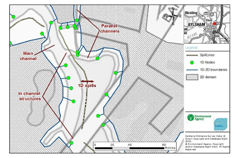
Example of multiple modelling approaches on the River Bure, Norfolk.
Initial conditions: how to include them in your model
Initial conditions are the starting conditions your model needs for an unsteady simulation. They’re estimates of channel or pipe network conditions that are usually needed to begin your simulation.
Initial conditions can include (among other variables):
- flow
- water level
- velocity
In most cases they should represent the normal channel condition. Depending on your modelling software, you may need to include an estimate of channel, pipe network or structural initial conditions. You’ll need to include these before you run the simulation.
You use other modelling software that does not need conditions specified to run. You can estimate initial conditions on a short model reach, possibly using hydraulic theory.
You can also generate them by carrying out a steady model simulation at low flows and using the results. As initial conditions are defined by boundary conditions, you may need to include manual alterations in some cases. For example, if there’s a known starting reservoir or tidal water levels.
If you use a pre-defined level, this will lead to instabilities in your model (for example, forcing a high tide level at time 0). It can be beneficial to run your model for a warm-up period. This will allow the boundary conditions to slowly ramp-up to the desired conditions before the arrival of a flood wave.
You can store initial conditions within the model file or in a separate file read into the simulation controls. If you use a separate file, you should supply it alongside the model.
You should check that initial conditions are sensible. If initial conditions were created during model development when instability was present, they may fluctuate throughout the reach. This could lead to ongoing instabilities or influence peak results. For example, if the initial condition water level is more than the the peak flow condition level.
Estimate hydraulic roughness
Hydraulic roughness is the measure of resistance water experiences when it passes through channels and over floodplains. In hydraulic modelling, roughness coefficients represent this resistance to flow.
Manning’s ‘n’ is the roughness coefficient that is typically used in the UK. Estimating a roughness coefficient using Manning’s ‘n’ or an equivalent is the main difficulty in hydraulic calculations according to the FDG.
Factors that can affect hydraulic roughness include:
- seasonal variations due to vegetation growth and die back
- maintenance procedures that can have a major impact if vegetation is cleared or channels dredged
You must consider the likely channel conditions expected during a flood event. Conditions can vary between catchments and should be agreed in the modelling method statement.
Estimate 1D hydraulic roughness
If the flow remains within channel, factors affecting hydraulic roughness can include:
- the bed and bank material
- channel and bed irregularity
- cross-sectional variation
- obstructions
- channel and bank vegetation
- variations in cross-sectional size and shape
The typical approach you should use for working out hydraulic roughness in 1D models was defined by Cowan (1956).
To estimate Manning’s ‘n’, values were attached to each factor that can affect hydraulic roughness:
- the bed and bank material (nb)
- channel and bed irregularity (n1)
- cross-sectional variation (n2)
- obstructions (n3)
- channel and bank vegetation (n4)
- variations in cross-sectional size and shape (m)
They then used the following equation: Manning’s ‘n’ = (nb+n1+n2+n3+n4) multiplied by m
Estimating Manning’s ‘n’ is a subjective process. To help you, various sources (Chow 1959, USGS, 1984 and Hicks and Mason, 2016) provide photographs of channel types for a given Manning’s ‘n’ value. These can help to provide a consistency of approach across different models. Refer to:
- V.T. Chow, ‘Open-channel hydraulics’ (1959)
- United States Geological Survey, ‘Guide for Selecting Manning’s Roughness Coefficients for Natural Channel and Floodplains’ (1984)
- Hicks and Mason, ‘Roughness Characteristics of New Zealand Rivers: A handbook for assigning hydraulic roughness coefficients to river reaches by the visual comparison approach’ (2006)
Hydraulic roughness ranges
Both the FDG and HEC-RAS provide guidance values for typical Manning’s ‘n’ values. They both range between a minimum value of 0.025 and a maximum value of 0.0150.
The Flood Modeller’s health checking utility also provides guidance values. However, this will return an error if Manning’s ‘n’ values are below 0.018 or above 0.100. It will return a warning if the values are less than 0.030 and more than 0.060.
Ranges can differ between different models and modellers. If you do not have very detailed calibration data it is not possible to determine an exact value. Therefore, appropriate ranges are often used during model review processes.
Fluvial Design Guide 1D hydraulic roughness ranges
The FDG provides a table of typical Manning’s ‘n’ values. This ranges from 0.025 (clean straight channel) to 0.150 (highly vegetated) for channels and 0.025 (short grass) to 0.200 (dense trees) for floodplains.
Table 3: The FDG’s typical Manning’s ‘n’ values for 1D hydraulic roughness ranges
| Channel description | Minimum Manning’s ‘n’ value | Maximum Manning’s ‘n’ value |
|---|---|---|
| Clean, straight, no riffles or deep pools | 0.025 | 0.033 |
| Clean, winding, some pools and shoals | 0.033 | 0.045 |
| Sluggish reaches, weedy, deep pools | 0.050 | 0.080 |
| Very weedy, deep pools | 0.075 | 0.150 |
HEC-RAS Manual 1D hydraulic roughness ranges
The typical values provided by the HEC-RAS manual differ in some places compared to the FDG.
Table 4: The HEC-RAS typical Manning’s ‘n’ values for 1D hydraulic roughness ranges
| Channel description | Minimum Manning’s ‘n’ value | Maximum Manning’s ‘n’ value |
|---|---|---|
| Clean, straight, no riffles or deep pools | 0.025 | 0.033 |
| Clean, straight, no riffles or deep pools but with more stones and weeds | 0.030 | 0.040 |
| Clean, winding, some pools and shoals | 0.033 | 0.045 |
| Clean, winding, some pools and shoals but with more stones and weeds | 0.035 | 0.050 |
| Sluggish reaches, weedy, deep pools | 0.050 | 0.080 |
| Very weedy, deep pools | 0.070 | 0.150 |
Hydraulic roughness for pipe networks
Colebrook-White is the most common hydraulic roughness coefficient for pipe network modelling. However, you can also apply Manning’s ‘n’, which is most relevant to large diameter pipes.
Sewers for Adoption 8 states that the design roughness for surface water and lateral drains should be 0.6mm and for foul sewers should be 1.5mm. Where no detailed information is available, you can provide these values. They should be updated to reflect pipe conditions where the information is available. Roughness typically ranges from 0.3mm for steel to 45mm for masonry pipes.
It is not necessary to provide excessive levels of detail when working out hydraulic roughness for pipe networks. For example, calculating values to 3 decimal places in locations with no calibration data.
Due to the significant uncertainty in estimating roughness on uncalibrated reaches, your estimates should be proportional. Avoid highly precise values without sufficient justification. Also, rapidly changing roughness values can lead to an illusion of accuracy.
2D hydraulic roughness
Your 2D roughness areas should vary depending on land use. This is typically informed by OS MasterMap datasets.
LIT11327: computational modelling to assess flood and coastal risk notes that reference sources are lacking for spatially varying 2D roughness coefficients, although some software manuals make recommendations.
It is suggested you run all 2D models for a ‘reference case’ with a model-wide value of 0.100 applied. You should compare results against spatially varying Manning’s ‘n’ values used in your design runs.
Project scopes rarely specify this requirement. They usually assess uncertainty via sensitivity tests. Project managers should consider adding this to project scopes. If your software allows application of depth-varying roughness values, higher roughness for shallow flows is recommended. This is relevant to direct rainfall modelling.
Your roughness values in 2D models should generally increase with model grid size. For that reason, it is not appropriate to provide typical ranges here, as these will vary depending on your other modelling decisions.
The FMRC in 2008 investigated the effect of using sub-grid scale hydraulic roughness (in coarse grid models) on inundation predictions. It was also referenced in SMFFLE.
The investigation used a case study on a densely urbanised London floodplain, TUFLOW 2D models were simulated using 2m, 10m and 50m numerical grids. Manning’s ‘n’ values were assigned at cell centres in the:
- 2m model, uniform values of 0.5 for buildings and 0.035 on floodplains
- 10m and 50m models, values according to n=0.035 + f(p) where p is the proportion of each cell occupied by buildings
The study calculated overall discrepancy indicators based on arrival times throughout the floodplain. They were compared with the results from the 10m and 50m models to the results from the benchmark 2m model. An optimised form for f(p) was determined (note: not provided in the accompanying documentation). The proposed parameterisation technique was found to improve results compared to a simpler method where roughness was assigned depending on land-cover type at cell centres. The improvement was typically one order of magnitude for the 10m model. For the 50m model a substantial improvement was observed, although it was less consistent than for the 10m model.
Modelling weir coefficients
You should consider whether default weir coefficients in modelling software for 1D structures are appropriate. Default values can be suitable for formal weirs but may need adjustment for less efficient structures such as rock weirs.
Software defaults typically assume that the unit is representing an in-channel structure. You’ll also need spill and weir units in 1D models to model flow:
- overtopping lateral embankments
- bypassing structures and structure decks
These are likely to represent less efficient flow paths than in-channel structures. There is limited hydraulic literature on the choice of coefficients for these structures. This means it is down to modeller experience with adjustments made to align with calibration data or anecdotal evidence.
Flood Modeller and InfoWorks-ICM historically used a default spill value of 1.7. The Flood Modeller manual describes this as suitable for a round nosed horizontal crested weir.
Flood Modeller has recently changed the default spill value to 1.2. This is to acknowledge the use of the spill unit for many structures that bear little resemblance to a round nosed weir.
Where the weir or spill is less efficient, the Flood Modeller manual states that the weir coefficient (Cd) value should be reduced.
It also states:
-
accurate guidance on the selection of Cd values for maintained grass embankments is not available although current good practice suggests values in the range 0.8 to 1.2
-
if the spill is being used to model flow over heavily overgrown natural ground, for instance, which is less efficient than a flood bank, then lower values may be applicable
In this scenario, you should alter the software defaults and justify the values adopted. They should be calibrated where possible. You may also be requested to carry out sensitivity testing to these coefficients.
Modelling downstream boundaries
Downstream boundaries are modelling components that allow water to leave both 1D and 2D model domains.
To represent downstream boundaries within hydraulic models in modelling software you can use:
- stage hydrography boundary
- flow hydrography boundary
- normal depth boundary
- flow-level boundary
The downstream boundary you choose will depend on the data you have, the location of the boundary and local characteristics.
If you are using uncertain data, your boundary should be a sufficient distance from your area or areas of interest. This will help to negate the impact of any assumptions you make.
Stage hydrography boundary
Stage hydrograph boundary is sometimes called a level-time or a head versus time (HT) boundary. It is a stage hydrograph of water levels versus time.
You can use it where the watercourse flows into a backwater environment, such as:
- an estuary
- an outfall where the downstream levels are governed by tidal levels
- scenarios where it flows into lakes or reservoirs of known stage
You can use a stage hydrography boundary to represent recorded gauge levels if you use it for an observed flood event.
If it is tidal, you’ll have to decide whether the peak model outflow should coincide with the high tide. This is part of a joint probability problem and what you propose should be outlined in your hydraulic modelling method statement.
Flow hydrography boundary
Flow hydrograph boundary is sometimes called a flow-time or QT boundary. It is a hydrograph of flow versus time. You can use it if recorded gauge data is available and the model is calibrated to a specific flood event. It is not used for modelling design flood events.
Normal depth boundary
Normal depth boundary is a type of boundary that automatically generates a flow-level relationship based on the bed or water surface slope. The relationship is calculated using the Manning’s ‘n’ equation. This is often the only choice available if the model reach does not finish at a gauge, confluence or tidal outfall.
Flow-level boundary
Flow-level boundary is sometimes called a rating curve, QH or HQ boundary. This boundary also uses a flow-level relationship, but unlike the normal depth boundary this is user-defined. The information for these boundaries can come from gauging station rating curves or extracted from existing models.
Placing a downstream boundary
You should carefully consider the placement of the downstream boundary. According to the FDG, the boundary should be sufficiently far from the site of interest so that it does not affect the results there.
You may be able to place the boundary closer to prevent the need for extensive topographic survey if it is hydraulically disconnected from the site of interest. For example, if it is downstream of a major weir.
Careful placement can negate the impact of uncertainty at the boundary. As a simple check, the distance between the site of interest and the boundary should exceed the backwater length (L). You can estimate this using the following formula: Backwater length = 0.7 multiplied by depth divided by gradient (m/m)
If the boundary is within a 2D domain, you should provide a sufficiently long boundary to include all flow paths leaving the model. This will prevent glass-walling.
You may have no choice where to place a boundary - for example, if the model discharges through a tidal flap. Assess any assumptions you make modelling the downstream boundary by sensitivity testing.
Request referenced documents
To request a copy of a document referenced in this guidance or a copy of the full PDF version of this guidance and the Microsoft Excel-based Fluvial Model Assessment Tool, email enquiries@environment-agency.gov.uk.
You should quote the reference number of the document you need, for example, LIT11327.