Research and analysis

Evaluating the impact of the 2017 Stamp Duty Land Tax First Time Buyers’ Relief

Published 31 May 2023

Summary

This paper estimates the efficacy of the 2017 First Time Buyers’ (FTB) Relief in incentivising FTB property transactions in England and Northern Ireland, as well as quantifying the impact of the policy on the prices paid by FTBs for property transactions.

The paper applies a Difference-in-Difference (DiD) Fixed Effect technique to Financial Conduct Authority (FCA) data, using home-mover (HM) transactions as the counterfactual across 2 discrete mortgage value bands of £125,001 to £300,000 and £300,001 to £500,000.

The results show that in the £125,001 to £300,000 band the relief resulted in an 11% increase in transactions over and above the volume of FTB transactions that would have taken place in absence of the policy.

Furthermore, the policy led to 1% increase in the prices that FTBs paid for property transactions in the same mortgage value band. In the £300,001 to £500,000 band the analysis finds an 18% increase in transactions over and above the volume of FTB transactions that would have taken place in absence of the policy. However, it did not derive a statistically significant impact on prices paid by FTBs in this mortgage value band.

The views expressed in this report are those of the authors and do not necessarily represent those of HMRC. Any remaining errors are the authors’ own responsibility.

Authors: R. Shopov, H. Howell, and F. Claridge

1. Introduction

On 22 November 2017, as part of the Autumn Budget, the Chancellor announced a permanent relief from SDLT for FTBs. The relief was a full exemption from paying Stamp Duty Land Tax (SDLT) for transactions at or below the value of £300,000 and property transactions taking place between £300,000 and £500,000, benefitting by a flat £5,000 relative to HMs. Above £500,000 there was no relief and the standard rates of SDLT applied.

This relief follows on from a similar temporary relief that was in action until 2012, which was also subject to an evaluation (Bolster, 2011). The key differences between the 2 policies are the thresholds to which the relief applies. The 2011 relief exempted FTB transactions from SDLT only for property transaction values up to £250,000, with normal rates applying from £250,001 onwards.

This evaluation has been commissioned as part of HMRC’s ongoing work to cost and review its existing tax reliefs. Inspiration was drawn from the published 2011 evaluation to arrive at the methodology used to assess against the objectives of the relief. Effort was made to use controls for macroeconomic, seasonal, and regional effects that mirrored the previous work, both for comparability and as a base on which to develop the methodology further.

DiD analysis is employed to assess the effects of the relief against a counterfactual. The model incorporates controls for the aforementioned external effects, isolating the impacts of the relief, thereby allowing for the estimation of how many additional FTB transactions occurred due to the policy, and the effect this had on average prices paid by FTBs.

2. Criteria for evaluation

The key objective of a SDLT relief for FTBs is to incentivise the purchase of properties through tackling the problems traditionally faced by this buyer type. The key issue of affordability is addressed by reducing the transaction costs associated with purchasing a property. In theory, this should result in greater numbers of FTB transactions due to the assumption that FTBs are relatively price elastic and should respond accordingly to a lowering of upfront transaction costs.

This evaluation looks at the below criteria to evaluate the success of this relief:

• the impact on transaction volumes of FTBs
• the impact on prices paid by FTBs

The impact on transactions is assessed as the number of transactions that are additional as a result of the relief. To effectively conduct this analysis, we needed information beyond the administrative data held by HMRC on the take-up of the relief, as we need to observe the period before the treatment (the introduction of the relief) in order to determine the magnitude of the effects of the treatment in the period after implementation. Data on the number of FTB transactions prior to the introduction of the relief is not held by HMRC.

To assess the impacts on prices paid by FTBs we need to again process data before and after the treatment. For the purposes of this analysis, we use a weighted average of transaction prices, whereby the average price in each price band is weighted by the number of transactions in the corresponding price band for a given Postcode Area (PA) and month within the sample.

This analysis will solely look to evaluate the impacts according to the above criteria and will not address any secondary effects that will translate into wider markets, or other indirect effects of the relief. The paper also does not examine the duration of the effects on transaction volumes and prices.

3. Data sources

Due to the specific requirements for this analysis, data was obtained from the FCA Mortgage Lending and Administration Return (MLAR) Statistics on the volumes of transactions undertaken by both FTBs and HMs (for example, non-first time buyers) from January 2012 to September 2019. The FCA also provided data on the average prices (median and mean) for both buyer types for the same time period.

The transactional FCA data was for mortgage transactions only, therefore excluding cash purchases. The data was provided on a monthly basis and was separated out into price bands of £25,000 intervals from £0 up to £525,000, with broader ranges used thereafter. The price bands provided are listed in Table 1:

Table 1: Price band breakdown of data (transactions and prices)

Price band
£0 to £100,000
£100,001 to £125,000
£125,001 to £150,000
£150,001 to £175,000
£175,001 to £200,000
£200,001 to £225,000
£225,001 to £250,000
£250,001 to £275,000
£275,001 to £300,000
£300,001 to £325,000
£325,001 to £350,000
£350,001 to £375,000
£375,001 to £400,000
£400,001 to £425,000
£425,001 to £450,000
£450,001 to £475,000
£475,001 to £500,000
£500,001 to £525,000
£525,001 to £925,000
£925,000 or greater

The data is provided on a PA geographical breakdown. There are 121 PAs in the UK (124 when taking into account the Crown Dependencies of Guernsey, Isle of Man, and Jersey, though the PAs for the Crown Dependencies were not used). Data was unavailable for FTBs in the West Central London (WC) PA, so this has been omitted from the analysis.

All PAs that capture regions of Scotland and Wales have been removed from the analysis. This is due to the fact that SDLT is devolved in both nations, and therefore the FTB relief does not apply to transactions within Scotland and Wales. In the case of Wales devolution occurred on 1 April 2018, meaning the treatment does not apply after the first 5 months of the post-treatment period. The removal of affected PAs results in removing some English PAs as their boundaries cross over into Wales and Scotland. We omit these as we do not have transaction level data in order to determine whether transactions in those PAs took place in England or in one of the devolved nations.

The FCA has censorship standards when sharing data, as such, for any price band in a given month, where the volume of transactions was 5 or less, these values have been censored. For the purposes of this analysis, we have treated these as missing values.

The treatment for the data on average prices is much the same, with the average prices provided only for the months and price bands where the values for transactions were not censored.

Data from UK Finance, Building Societies Association, and the Office for National Statistics (ONS) was also used to compile the macroeconomic controls used in both the transaction and price equations.

4. Methodology

There are a number of factors that have significant impacts on both transaction volumes and average prices in the housing market. Many of these factors are difficult to measure and observe. To isolate the effect of the FTB relief on both of these metrics this paper will employ a DiD methodology. The key assumption of parallel trends of the treatment and control groups will, if proven to hold, ensure that any unobserved effects driving trends in the time series will be controlled for. This combined with the controls for macroeconomic factors, seasonal, and regional effects will allow the model to better isolate the impact of the relief, and mitigate the effects of any bias caused by unobservable factors.

Inspiration was taken from Bolster 2011 for the specification of the model, with effort made to assemble macroeconomic controls that are closely aligned to those used in the previous evaluation. This paper then looks to build on this basis, with adjustments made to the model specification to account for overspecification and multicollinearity that exists between a number of the original factors used in Bolster 2011. The reasoning for these is discussed in section 4.6.

4.1. Sample period

The analysis in this paper has been conducted using monthly data from October 2016 to November 2018. This allows for a 13-month pre-treatment period, and an equivalent 13-month post-treatment period. Using a longer pre-treatment period would have resulted in potentially having to control for the introduction of other SDLT policies, adding uncertainty and complexity to the model.

4.2. Treatment and control groups

This analysis will focus on the effect of the FTB relief on transactions and average prices paid by FTBs in the relieved price band, £125,001 to £500,000. This sample is then broken down into 2 further groups based on the extent of relief within the price bands, £125,001 to £300,000 and £300,001 to £500,000. This was done as the Effective Tax Rates (ETRs) will differ between the 2 groups, where ETR is the tax paid divided by the value of the property. This allows us to compare the relative changes in tax for differently priced properties. The effect of the relief is expected to be greater for the group £300,001 to £500,000 since their ETR is decreased on average by a greater magnitude than that of the £125,001 to £300,000 group. The variance in the sample sizes between the 2 groups would also mean that the group specific elasticities of the larger sample would contribute more to the overall elasticity estimate, and as such we took the judgement that presenting the 2 price groups separately would more accurately illustrate the effects of the relief. Sensitivity analysis in Appendix 2 shows the results of pooling the price groups.

For the purposes of the analysis the treatment group is FTBs, as this is the buyer group targeted by the relief. The control group will be HMs within the relieved price bands indicated above. The choice of control was driven by the availability of data.

Another potential control that was considered is FTBs that undertook transactions at £125,000 or less. However, due to missing values in a majority of the PAs, non-relieved FTBs were not a viable control group. Furthermore, the model adopted in this paper uses natural logarithms, and since it is not possible to take the natural logarithm of 0, any PAs which contained at least one value of 0 for any given month were removed from the data for the entire period of the analysis to ensure a balanced panel. Furthermore, the limited supply of housing below £125,000, particularly in certain regions, suggests that this group would be too different to the treatment group, and so would not offer a robust counterfactual. Therefore, the best available control group for the analysis was HMs within the relieved price ranges.

Despite this, it was possible to conduct sensitivity analysis for transactions and prices, in the £125,001 to £300,000 price group, using FTBs that undertook transaction at £125,000 or less as the counterfactual. This was used as a way to assess the results of the main analysis and is discussed further in the Appendix 1.

Below is a table outlining the respective sample sizes, represented by number of PAs, for the transaction and price datasets:

Table 3: Number of PAs in sample datasets for transaction and price analyses

Number	£125,0001 to £300,000	% of UK PAs	£300,001 to £500,000	% of UK PAs
Transactions	73	60.3%	31	25.6%
Price	73	60.3%	31	25.6%

The £125,001 to £300,000 analysis is based on data from 73 PAs which make up ~60% of all UK PAs, excluding Crown Dependencies. The £300,001 to £500,000 analysis is based on data from 31 PAs, which account for ~26% of all UK PAs, excluding Crown Dependencies.

4.3. DiD analysis

DiD analysis is the comparison of 2 distinct periods of data: the period before the treatment (in this case the period prior to the introduction of the SDLT FTB relief), and the period after the treatment. A stylised example below helps to illustrate the theoretical foundations of the methodology.

Chart 1: DiD illustrative example

Chart 1 above shows the transaction volumes for both FTBs (treatment group) and HMs (control group). For the purposes of the example, it is assumed that the introduction of the relief increases the transaction volumes of FTBs. There are 2 distinct time periods, Period A which is the pre-treatment period, and Period B, the post-treatment period.

Period A illustrates the theory of the parallel trends assumption. This is shown by the similarity between the trends for HMs and FTBs. These trends are due to unobservable factors. If the assumption of parallel trends holds then these unobservable factors will not influence the results of our analysis, as the difference between the 2 groups would remain constant in the absence of treatment.

In period B, given that the parallel trends assumption holds, we project forward the pre-intervention trend for the treatment group. This provides an estimate for what the level of transactions would have been for FTBs in the absence of the relief (shown by the orange line). This is then compared to the actual levels of FTB transactions, the difference between the projected pre-intervention level and the actual level provides the DiD estimator for the impact of the relief on FTB transactions.

4.3.1. DiD box analysis

As in Bolster 2011, this basic methodology can be applied on the aggregate level data for England and Northern Ireland to provide some initial estimates as to the effect of the relief on both transactions and prices. Tables 4 to 7 display these estimates:

Table 4: DiD analysis: £125,001 to £300,000 group – aggregate average transactions volumes

Date	Before November 2017	After November 2017	Difference between periods
FTBs in £125,001 to £300,000 price range	11,781	12,530	750
HMs in £125,001 - £300,000 price range	10,891	10,614	-277
Difference between groups	889	1,916	1,027
Estimated transactions in absence of relief	–	11,503	–
Estimate of additional transactions	–	–	1,027
Estimated percentage increase	–	–	8.9%

Table 5: DiD Analysis: £300,001 to £500,000 group – aggregate average transaction volumes

Date	Before November 2017	After November 2017	Difference between periods
FTBs in £300,001 to £500,000 price range	2,656	2,937	281
HMs in £300,001 to £500,000 price range	3,603	3,526	-76
Difference between groups	-947	-590	357
Estimated transactions in absence of relief	–	2,579	–
Estimate of additional transactions	–	–	357
Estimated percentage increase	–	–	13.8%

Table 6: DiD analysis: £125,001 to £300,000 group – aggregate average prices (£)

Date	Before November 2017	After November 2017	Difference between periods
FTBs in £125,001 to £300,000 price range	190,387	194,567	4,180
HMs in £125,001 to £300,000 price range	220,230	222,733	2,503
Difference between groups	-29,842	-28,165	1,677
Estimated transactions in absence of relief	–	192,890	–
Estimate of additional transactions	–	–	1,677
Estimated percentage increase	–	–	0.9%

Table 7: DiD analysis: £300,001 to £500,000 group – aggregate average prices (£)

Date	Before November 2017	After November 2017	Difference between periods
FTBs in £300,001 to £500,000 price range	361,360	364,651	3,290
HMs in £300,001 to £500,000 price range	400,153	402,246	2,092
Difference between groups	-38,793	-37,595	1,198
Estimated transactions in absence of relief	–	363,453	–
Estimate of additional transactions	–	–	1,198
Estimated percentage increase	–	–	0.3%

This basic analysis was carried out on the same sample period that is used throughout the paper, October 2016 to November 2018, allowing for equivalent 13-month periods either side of the relief being introduced in November 2017.

Averages were taken for the pre- and post-treatment periods. The difference between these periods is then computed, showing the difference between the averages for FTBs before and after the introduction of the relief. However, to ascertain the true effect of the relief, unobservable factors that may be driving the changes in the results also need to be controlled for. As such, the difference between the 2 periods is also estimated for the control group, HMs. Under the parallel trends assumption, which underpins DiD methodology, we assume that the difference between these differences is due to the treatment, the introduction of the relief on FTBs.

To estimate the percentage change in transactions and prices as a result of the relief an estimate of the transactions/prices in the absence of the relief must be obtained. This is done by taking the figure for HMs in the post-treatment period and adding the magnitude of the difference between the 2 buyer groups in the pre-treatment period. This provides an estimate of the FTB transaction volumes/price levels in the absence of the relief. The estimated additional transactions/price increases are then divided by this figure to give an estimate of the percentage increase as a result of the relief.

The aggregate level calculations in the tables above provide transaction impact estimates of 8.9% and 13.8% for the £125,001 to £300,000 and £300,001 to £500,000 mortgage value bands, respectively. The price impact estimates are 0.9% and 0.3% for the £125,001 to £300,000 and £300,001 to £500,000 mortgage value bands, respectively.

4.3.2. The DiD equation

Translating the above theory into an analytical model yields the following equation:

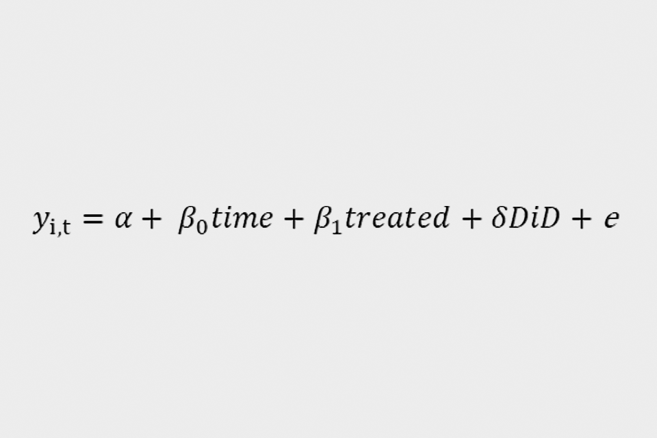
Where ‘y’ is the dependent variable upon which the treatment has had an effect (transaction volumes/prices), ‘a’ is a constant term, ‘time’ is a dummy variable that equals 0 in the pre-treatment period and 1 in the post-treatment period, ‘treated’ is a dummy variable which equals 1 for the treatment group (FTBs) and 0 for the control group (HMs), ‘DiD’ is an interaction term equal to ‘time’ multiplied by ‘treated’, the coefficient for this variable represents the DiD estimator, which is the impact of the treatment. ‘e’ is the error term.

Whilst a very useful tool for basic analysis and controlling for unobserved effects, the above equation does not control for outside factors that can also be driving the changes in transaction volumes and average prices, and therefore impact our treatment and control group differently. Economic variables such as the cost of borrowing, mortgage availability and GDP are among some of the macroeconomic factors that could potentially be driving the change. By taking the averages of England and Northern Ireland totals of transactions/prices over 2 13-month periods, the above analysis does not control for variation caused by seasonal and regional effects. This results in this specification being an insufficiently robust method for ascertaining the true impact of the relief on transactions and prices.

The next sections will discuss the expansions made to the specification of the basic DiD model in order to produce more accurate estimates of the policy impact on transactions and prices.

4.4. The DiD equation: transactions

The DiD model that will be used for the analysis into transactions has its foundations in Bolster 2011. An effort was made to mirror the macroeconomic controls used in the previous paper. These were then incorporated into the basic DiD equation, along with quarterly dummy variables in order to control for seasonal effects, and dummy variables for the PAs contained within each dataset. Once these additional controls have been incorporated into the basic DiD equation the analytical model is as follows:

Where ‘yi,t’ is the log of the number of transactions of buyer type ‘i’ at time ’t’, and ‘Xi,t’ are the macroeconomic controls for buyer type ‘i’ at time ’t’. ‘a’ and ‘B’ are the constant and the coefficient that are being estimated, respectively. ‘e’ is the error term.

Table 8 details the additional controls that will be introduced for the transaction analysis. The average standard variable mortgage rate and the GDP growth variables capture the income and GDP growth expectations of prospective buyers. Net new mortgage advances, median income multiple, and median loan to value ratio control for changes in the volume of mortgage approvals, as well as controlling for any potential impacts caused by the differential in sensitivities to credit restrictions faced by FTBs and HMs. The quarterly dummy variables are included to control for any seasonal effects, and the PA dummy variables control for the impacts of regional differences.

The equation was run on data at a PA level of granularity, for the sample period outlined in 4.1, October 2016 to November 2018, for both price groups, £125,001 to £300,000 and £300,001 to £500,000. In total, the analysis is conducted on 3,796 observations for the £125,001 to £300,000 price group, and 1,612 observations for the £300,001 to £500,000.

Table 8: Variable descriptions – additional controls for transactions equations

Variable	Source
Log monthly average standard variable mortgage rate	Building Societies Association. The data source used in Bolster 2011 was not available.
Log (t-1) monthly net new mortgages, lagged by 1 year to account for potential endogeneity	UK Finance Table MM13
Log monthly income multiple by buyer type (mean)	UK Finance Tables RL1&2. Bolster 2011 used the median average of this metric, however UK Finance changed their reporting practises from median to mean.
GDP growth - quarter on quarter growth rate from same quarter in previous year	ONS (code ABMI)
Q2, Q3, Q4	Quarterly dummies to control for seasonal effects
PAd	PA dummies for each data set d, to control for regional effects.

4.5. The DiD equation: prices

DiD methodology is, again, employed in the analysis of the price effects of the relief. Inspiration for the specification is again taken from Bolster 2011, though some deviations were made, the reasons for which are explained in section 4.6.

The additional macroeconomic, seasonal, and regional controls, which were added to the basic DiD equation, are detailed in Table 9. As before, the average standard variable mortgage rate and the GDP growth variables capture the income and GDP growth expectations of prospective buyers. Net new mortgage advances, median income multiple, and median loan to value ratio control for changes in the volume of mortgage approvals, as well as controlling for any potential impacts caused by the differential in sensitivities to credit restrictions face by FTBs and HMs. The additional variable, of quarterly real gross non-property disposable income captures the effects of an income differential between FTBs and HMs on the prices of transactions. The quarterly dummy variables are included to control for any seasonal effects, and the PA dummy variables control for the impacts of regional differences. These additions to the model result in the following specification of the DiD equation:

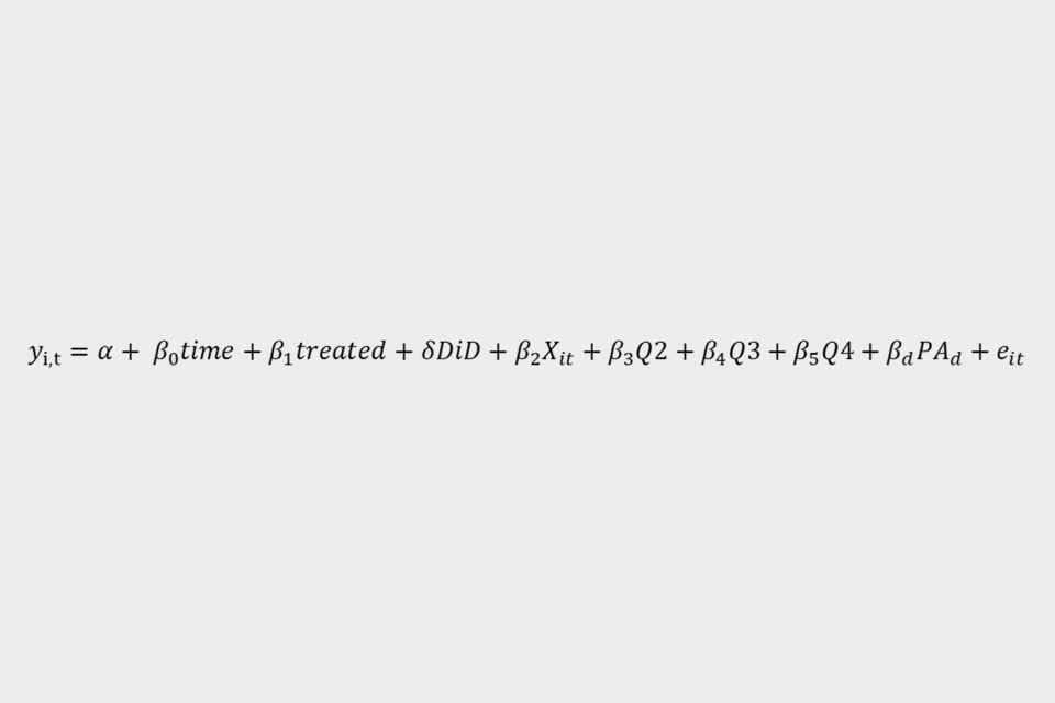
Where ‘yi,t’ is the log of the average price of buyer type ‘i’ at time ‘t’, and ‘Xi,t’ are the macroeconomic controls for buyer type ‘i’ at time ‘t’. ‘a’ and ‘b’ are the constant and the coefficient that are being estimated, respectively. ‘e’ is the error term.

The equation was run on data at a PA level of granularity, in the sample period outlined in section 4.1, October 2016 to November 2018, for both price groups, £125,001 to £300,000 and £300,001 to £500,000.

Table 9: Variable descriptions – additional controls for price equation

Variable	Source
Log monthly average standard variable mortgage rate	Building Societies Association. The data source used in Bolster 2011 was not available.
Log (t-1) monthly net new mortgages, lagged by 1 year to account for potential endogeneity	UK Finance Table MM13
Log monthly income multiple by buyer type (mean)	UK Finance Tables RL1&2. Bolster 2011 used the median average of this metric, however UK Finance changed their reporting practises from median to mean.
GDP growth - quarter on quarter growth rate from same quarter in previous year	ONS (code ABMI)
Log quarterly real gross non-property disposable income	Constructed using ONS data (codes: NRJR, ROYL, D7BT)
Q2, Q3, Q4	Quarterly dummies to control for seasonal effects
PAd	PA dummies for each data set ‘d’, to control for regional effects

4.6. Model specification

The keen reader will notice that there are differences between the macroeconomic controls that form part of the models in this paper and those used in Bolster 2011. These differences are present in the equations for both the transactions analysis and price analysis. Below is a discussion of the reasons behind these adjustments.

4.6.1. Transactions

The starting point for this analysis was to run the DiD equations and to include identical macroeconomic controls to Bolster 2011. The key differences between this and the model used in this paper, is that Bolster’s equation contained controls for the loan-to-value ratio by buyer type, and the lagged dependent variable.

The choice to omit the control for the loan-to-value ratio by buyer type was driven by tests conducted to check for overspecification of the model and the presence of multicollinearity. The first test was to look at the Variance Inflation Factor (VIF) of each variable. The VIF provides an index that measures how much the variance of an estimated regression coefficient is increased by multicollinearity. Of all the variables in the original Bolster 2011 equation the variables with the highest VIF critical values were the control for the income multiple by buyer type and the control for the loan to value ratio by buyer type, indicating that both of the coefficient estimates for these variables were being influence by collinearity.

The next step was to look at a correlation matrix of all the variables within the equation, to see whether there were any variables that presented with a high correlation with each other. The results mirrored those of the VIF index, showing that the control for the income multiple by buyer type was 94.2% correlated with the treated variable, and that the control for the loan to value ratio by buyer type was 99.6% correlated with the treated variable. The 2 variables were also highly correlated with each other, at 95.3%. The decision to exclude the control for the loan to value ratio by buyer type from the equation was made due to the near perfect multicollinearity with the treated variable. Furthermore, the high correlation between the income multiple by buyer type and the control for the loan to value ratio by buyer type suggests that the 2 variables are picking up a high proportion of the same effect, so removing the control for the loan to value ratio by buyer type does not significantly reduce the predictive power of the model.

The decision to omit the lagged dependent variable was taken to avoid overspecification. The justification provided by Bolster 2011for including a lagged dependent variable is to control for the impacts of time-invariant factors. However, since the analysis employs a fixed effects model, inherent to which is the mechanism for controlling for time-invariant effects, adding in the lagged dependent variable control will essentially duplicate this effect, removing a lot of the variation, and therefore introducing downward bias into the DiD coefficient. Hence, the decision was made to omit this variable from the transaction equation.

4.6.2. Price

The adjustments made to the model used to estimate the price effects echo those made for the transactions model. VIF indices and correlations were calculated for the variables with the same conclusion reached, to exclude the control for the loan to value ratio by buyer type from the model due to its near perfect collinearity with the treated variable, and its high correlation with the control for the income multiple by buyer type. The lagged dependant variable was also omitted from the price equation, for the same reasons as those listed above.

There were however changes made to the specification beyond the omission of the control for the loan to value ratio by buyer type and the lagged dependent variable. In Bolster 2011 the variables Log (t-1) monthly net new mortgages and GDP growth were omitted. The analysis presented in this paper reversed this decision, as the inclusion of these variable improved the predictive power of the model without introducing additional collinearity.

4.7. Parallel trends assumption

As mentioned throughout, a key assumption that underpins DiD methodology is the parallel trends assumption. This states that in the absence of treatment, the data needs to show that the trends between our treatment and control groups is relatively consistent for both transactions and prices to ensure that the results produced by the analysis are robust.

Given the importance of this assumption, there needs to be at least some degree of confidence that the assumption is valid for the data the analysis is based on. Whilst there is no standard test for the parallel trends assumption, it was the intention of this paper to conduct tests in order to prove with a high degree of confidence that the trends between treatment and control groups were indeed parallel.

The preferred method would involve running placebo regressions on pre-treatment data, the rationale being that in the absence of the policy the regressions would not identify any statistically significant treatment effects.

Unfortunately, it was not possible to conduct this level of testing. The main issue was the underlying data on which the test was conducted. Information from the FCA details that prior to July 2015 the purchase price was not a mandatory requirement for their reporting. Therefore, it is known that a transaction took place in a certain PA, in a certain month, however the price at which it went through was not known so there are a number of transactions that are not allocated to one of the £25,000 price bands. From later periods there were SDLT policies which made the changes unsuitable to use as a dummy dataset. This rendered our intended available back-series of data beyond the current pre-treatment period unusable, as any results would suffer from high magnitudes of bias.

As such, for the purposes of presenting an argument for the parallel trends assumption holding for this analysis we revert to the convention of inspecting the graphed UK totals for each sample. From charts 2 to 5 it is clear that the trends between FTBs and HMs, whilst not perfectly parallel, have great degree of similarity over time. The trends for the total transaction volumes have a greater degree of parallelistic inclination. This is confirmed by the correlation coefficients, 99% and 93% for the £125,001 to £300,000 and £300,001 to £500,000 data groups, respectively.

The correlation coefficients for the Average Prices tell a slightly different story, at 89% and -2% for the £125,001 to £300,000 and £300,001 to £500,000 data groups, respectively. This implies that we are not able to draw conclusions on the price effects in the upper price group. The low negative correlation implies that the average prices for FTBs and HMs move in opposite directions prior to the policy implementation, meaning it is not possible to isolate the specific treatment effect of the policy.

Chart 2: Plot of total transaction – £125,001 to £300,000 (October 2016 to November 2018)

Chart 3: Plot of total transaction – £300,001 to £500,000 (October 2016 to November 2018)

Chart 4: Plot of total prices – £125,001 to £300,000 (October 2016 to November 2018)

Chart 5: Plot of total prices – £300,001 to £500,000 (October 2016 to November 2018)

5. Empirical results

5.1. Impact on FTB transactions

The results of the analysis into the effect of the SDLT relief on FTB transaction volumes are outlined below in Tables 10 and 11 for the price groups £125,001 to £300,000 and £300,001 to £500,000, respectively. The equations reported are (1) the basic DiD equation; (2) model including variables omitted from final analysis; and finally (3) the model that this paper posits to be the most appropriate and robust estimate of the impacts of the relief.

Table 10: Estimated additional FTB transactions – £125,001 to £300,000 price range

Equation	DiD coefficient	Standard error	p-value	Adjusted R-squared
1. Basic DiD	0.1094	0.042557	0.01019	0.9%
2. DiD + omitted variables	0.0351	0.0149058	0.0187236	87.7%
3. Final model	0.1073	0.020364	1.463e-07	76.8%

Table 11: Estimated additional FTB transactions – £300,001 to £500,000 price range

Equation	DiD coefficient	Standard error	p-value	Adjusted R-squared
1. Basic DiD	0.1778	0.068508	0.009543	3.7%
2. DiD + omitted variables	0.0454	0.0316615	0.1519692	78.8%
3. Final model	0.1753	0.0485716	0.0003178	50.4%

Using our final model the estimated increase in FTB transactions as a result of the introduction of the SDLT relief can be reported as 10.73% for mortgage transactions in the £125,001 to £300,000 price range, and 17.53% for mortgage transactions in the £300,001 to £500,000 price range. The results for both mortgage value bands were statistically significant at the 1% level. The results show a decrease in the Adjusted R-squared when moving from model (2) to (3), however this can largely be explained by the omission of the lagged dependent variable as this would inherently increase the explanatory power of the model, given it contains the past moments of the dependent variable in question.

The difference between the model which includes the omitted variables in (2) and the final model (3) is the exclusion of the log of loan to value ratio variable and the lagged dependent variable. The reasoning for this was discussed in depth in section 4.6. From the above results, there is a marked difference in the treatment effects estimated by models (2) and (3). This is largely driven by the omission of the lagged dependent variable, and the effect this has on increasing the variation within the model.

5.2. Impact on prices paid by FTBs

The effects of the SDLT relief on mortgage transactions prices paid by FTBs are outlined below in Tables 12 and 13, for the £125,001 to £300,000 and £300,001 to £500,000 price groups, respectively. As for transactions, the results of 3 models are reported: (1) the basic DiD equation; (2) model including variables omitted from final analysis; and finally (3) the final model that this paper reasons as the most appropriate.

Table 12: Estimated impact of average price paid by FTBs in the £125,001 to £300,000 price range

Equation	DiD coefficient	Standard error	p-value	Adjusted R-squared
1. Basic DiD	0.0106	0.0083692	0.2069	24.3%
2. DiD + omitted variables	0.007	0.00211882	0.0009693	95.1%
3. Final model	0.0104	0.002286	4.80e-06	94.4%

Table 13: Estimated impact of average price paid by FTBs in the £300,001 to £500,000 price range

Equation	DiD coefficient	Standard error	p-value	Adjusted R-squared
1. Basic DiD	0.0039	0.0056294	0.4936	44.3%
2. DiD + omitted variables	0.0033	0.00302294	0.2756404	83.8%
3. Final model	0.0037	0.00308385	0.2316012	80.1%

The results above show that the introduction of the relief has led to an increase in the average prices paid by FTBs for mortgage transactions. The final model estimates that prices paid by FTBs in the £125,001 to £300,000 group increased by 1.04%, statistically significant at the 1% level, as a result of the relief. The estimate of the price impact for the £300,001 to £500,000 group shows an increase in the price paid by FTBs of 0.37%, however we see that the coefficient estimate is not statistically significant at the 20% level. A key driver of this issue is likely to be the weak parallel trends for the £300,001 to £500,000 price sample, which will mean that we cannot draw robust inferences from analysis on this portion of the data.

A drop off in the Adjusted R-squared can also be seen in the price impact estimates between models (2) and (3). As with results reported for the treatment effect on FTB transactions, the omission of the log of loan to value ratio and the lagged dependent variables lead to a difference in the reported coefficients for models (2) and (3) for the price effect on FTB transactions. This difference is once again largely attributable to the increase in the variation, which comes about from excluding the lagged dependent variable.

5.3. Comparison of results

Previous evaluations of a relief from SDLT for FTBs have been conducted by HMRC (Bolster 2011) so it is useful to reflect on the results obtained through this analysis in comparison to those previously derived.

The previous evaluation estimates were based on a different underlying SDLT structure, a slab structure where SDLT was paid on the price of the property, whereas the relief that is the subject of this paper is based on a slice structure, which is a marginal tax system. As such the tax change under the previous relief was different in magnitude to the current relief, and so we adjust our coefficients to ensure a consistent basis for comparison.

The adjustment is done using the following equation:

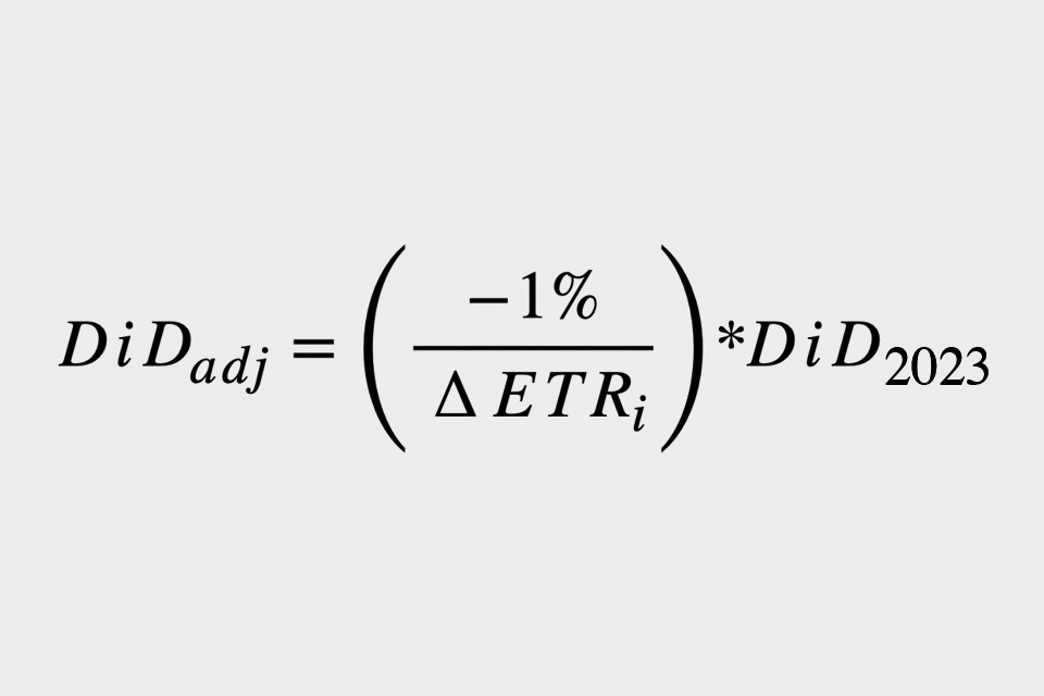
Where ‘DiD adj’ is the adjusted coefficient, ‘DiD 2023’ is the coefficient estimate derived in this paper, and ‘Delta ETR’ is the average change in the effective tax rate for the average price paid in each of the 2 price groups, £125,001 to £300,000 and £300,001 to £500,000, respectively.

The adjusted coefficients of the final models are presented below:

Table 14: Adjusted model coefficients

Amounts	‘DiD 2023’	‘Delta ETR’	‘DiD adj’
Transactions - £125,000 to £300,000	0.1073	-0.82%	0.1303
Transactions - £300,000 to £500,000	0.1753	-1.25%	0.1402
Price - £125,000 to £300,000	0.0104	-0.82%	0.0126
Price - £300,000 to £500,000	0.0037	-1.25%	0.0030

Bolster 2011 reports that FTB transactions increased by 2% due to the relief, and a 0.7% increase in prices paid by FTBs, when accounting for Local Authority fixed differences.

The treatment effects presented in this analysis, even when adjusted to be comparable with Bolster 2011, are significantly higher, particularly for the transaction impact estimates. This could imply a greater effectiveness of the 2017 FTB relief policy compared to its 2010 predecessor. However, drawing such a conclusion could be misleading.

Whilst this paper has taken great care to replicate aspects of the Bolster 2011 methodology in estimating the treatment effect, there are key factors which could go some way to explain the difference in results. Firstly, the economic climate of post-Financial Crisis 2010 could potentially have led to an under-provision of mortgage lending making it even more difficult for FTBs to purchase property. Secondly, whilst the macroeconomic controls used in this analysis were constructed to resemble those used in Bolster 2011, the controls have changed since the publication of the previous analysis. Namely the income multiple control variable, the reporting for which has shifted from a median to a mean average since 2011. Finally, the modifications to the model specifications will also be a driver for the difference in results, as the specification deployed in Bolster 2011 uses variables that this analysis has chosen to omit, for reasons provided in Section 4.6.

Therefore, the comparison of the results within this paper are aimed at showing the impact estimates of the 2 papers on a consistent basis, rather than to make a judgement on how the 2 policies compare.

5.4. Diagnostics

The Breusch-Pagan test was run on all the models used for the analysis, revealing the presence of heteroskedasticity. As a result, the coefficients are reported with White’s robust standard errors. The Augmented Dickey-Fuller test for unit root was run on the dependent variables for transactions and price. The null hypothesis was rejected at the 1% level of significance, indicating stationarity. The Durbin-Watson test was used to test for autocorrelation, the test failed to reject the null hypothesis of no first order correlation.

Appendix 1: Non-relieved FTBs as the control group

The result from the sensitivity analysis conducted on £125,001 to £300,000 price group with FTBs in the £0 to £125,000 price group are presented below in Tables A1 and A2. Results for the pooled analysis are shown in Tables A3 and A4. The results reported are for all specifications used for transactions and prices, respectively.

Table A1: Estimated additional FTB transactions in the £125,001 to £300,000 price range, with FTBs in the £0 to £125,000 price group as the counterfactual

Equation	DiD coefficient	Standard error	p-value	Adjusted R-squared
1. Basic DiD	0.1566	0.060354	0.009533	21.8%
2. DiD and omitted variables	0.021	0.0211953	0.3208301	90.2%
3. Final model	0.1566	0.04179	0.000183	62.6%

Table A2: Estimated impact of average price paid by FTBs in the £125,001 to £300,000 Price Range, with FTBs in the £0 to £125,000 group as the counterfactual

Equation	DiD coefficient	Standard error	p-value	Adjusted R-squared
1. Basic DiD	0.027	0.0067229	6.247e-05	92.3%
2. DiD and omitted variables	0.0108	0.003734	0.003826	97.7%
3. Final model	0.0269	0.004887	4.13e-08	96%

This analysis presents higher impacts on the number of FTB transactions in the £125,001 to £300,000 group of 15.66%, and a higher average price effect of 2.69% than the those presented when HMs are used as the control group. Though the model specification looks to control for regional difference through the use of PA dummies, it may be the case that differences in characteristics between the control and treatment group in this analysis, that are not being controlled for by any of the current variables within the model, are driving the difference in the sensitivity estimates from the main model results.

Appendix 2: Pooled price groups

The result from the pooled price groups analysis shows lower treatment effects on both number of transactions of 9.08% and average price of 0.51%.

Table A3: Estimated additional FTB transactions – £125,001 to £500,000 price range

Equation	DiD coefficient	Standard error	p-value	Adjusted R-squared
1. Basic DiD	0.0931	0.043752	0.0334634	0.2%
2. DiD and omitted variables	0.0365	0.014933	0.0145368	88.2%
3. Final model	0.0908	0.01966	3.93e-06	79.9%

Table A4: Estimated impact of average price paid by FTBs in the £125,001 to £500,000 price range

Equation	DiD coefficient	Standard error	p-value	Adjusted R-squared
1. Basic DiD	0.0051	0.0156984	0.74765	19.1%
2. DiD and omitted variables	0.0035	0.00246659	0.1575346	98%
3. Final model	0.0051	0.002657	0.057356	97.7%

A potential explanation is that compiling the dataset resulted in a greater number of PAs being incorporated into the analysis. This is because the datasets used for our main estimates omit PAs with at least one value of 0 for average price in the sample period. However, averaging from £125,001 rather than £300,001 means that even PAs where we do not have figures in the upper price group are being included in the analysis, which could potentially be introducing downward bias, as the transaction and price effects are being artificially dampened by the presence of what would be lower average values across the £125,000 to £500,000 range for those PAs.

Appendix 3: Prices weighted by the previous year’s transactions

The purpose of this sensitivity analysis is to attempt to isolate the price effect of the relief by abstracting from the transaction effect, which will itself contribute to the overall increase in the average prices of mortgage transactions.

The main analysis weights average price by the transactions in each price band by the corresponding transactions in the same month. For this analysis, the average price in the months following the policy introduction is weighted by the transactions in the corresponding month of the previous year. For example, average prices in October 2018 are weighted by the transactions in October 2017, rather than October 2018 as is the case in the main analysis.

This serves to show what the price impact generated by the relief would be had transactions not increased. The transaction effect estimates are unaffected by this analysis. The results of the price analysis are reported below:

Table A7: Estimated impact of average price paid by FTBs in the £125,001 to £300,000 price range

Equation	DiD coefficient	Standard error	p-value	Adjusted R-squared
1. Basic DiD	0.0142	0.0094947	0.1355	20.2%
2. DiD and omitted variables	0.0106	0.0046118	0.0219493	81.1%
3. Final model	0.0142	0.0047231	0.0026542	79.9%

Table A8: Estimated impact of average price paid by FTBs in the £300,001 to £500,000 price range

Equation	DiD coefficient	Standard error	p-value	Adjusted R-squared
1. Basic DiD	0.014	0.0141261	0.3234	18.4%
2. DiD and omitted variables	0.01	0.0121101	0.4103476	38%
3. Final model	0.0139	0.0128514	0.2809366	30.8%

In both price groups the estimated impact of the relief on prices paid by First Time Buyers is higher than in the main analysis with an estimate of a 1.42% increase in prices paid in the £125,001 to £300,000 price group, and 1.39% for the £300,001 to £500,000. As with the original analysis we do not obtain statistically significant estimates of the price effect for the £300,001 to £500,000 price group. However, the estimate for the price effect in the £125,001 to £300,000 group is now only statistically significant at the 1% level.

This analysis, whilst useful, only offers an approximation of the price effect in the absence of the transaction effect caused by the relief. It is not currently possible to fully disaggregate the magnitude of these 2 effects with the available data, and so the reported estimates of the sensitivity analysis should be treated only as indicative.